DX-Pedition to Rarotonga, Cook Islands

I will be active from Rarotonga, Cook Islands  IOTA OC-013  from April 1 to April 13, 2013.
This DX-pedition will be mostly a vacation but I hope to make a few contacts as well.  My call sign will be E51DXX and I will be working mostly SSB and digital modes.  I created this filter in DX cluster to check for possible spots.

I used VOACAP propagation planner and online tools to predict propagation from Rarotonga to various other  locations.  As a starting point I made some assumptions on antennas and transmit power.  I will carry a Buddipole antenna and two radios (Flex3000 and Elecraft KX3) with me.  Prediction was done assuming 100W transmit power, vertical antenna  and SSB transmit mode from Rarotonga.  For the other stations I assumed 3 element Yagi at 50ft and 100W.

The propagation prediction tables below show that 20M, 17M and 15M HF bands look like the most promising bands this time of the year.  The tables show the % probability of the contact and estimated S-unit signal strength for each ham band  over 24 hours (Raro / UTC timezones).  The best case to US East coast will be S4 signal strength and 28% probability at 20M  @07:00 UTC so bare with me and follow the DX Code of Conduct please.

I will be working mostly between 18 - 24 Rarotonga time which is 4:00 - 10:00 UTC.   Let's see how well this propagation prediction will match with reality.

I hope to make a QSO with you from Rarotonga, Cooks Islands.  Thanks for reading this blog. Feel free to leave feedback below.

73
Mauri AG1LE


Here is the CQ Zone map for reference (from EI8IC website).

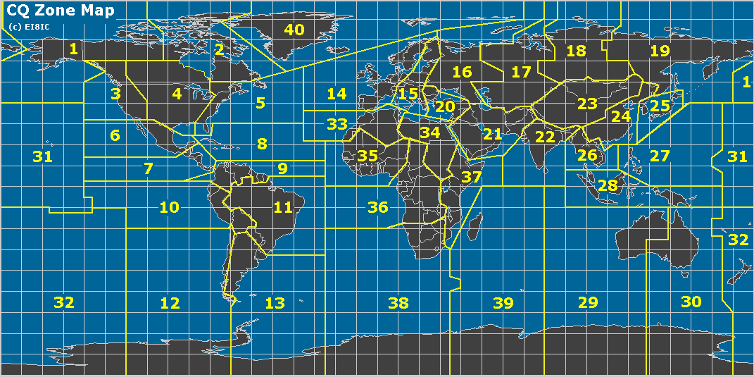
Figure 1.  CQ Zone Map  by EI8IC 

For CQ Zone 5  - US East Coast 

Raro	UT	80M	40M	30M	20M	17M	15M	12M	10M
15	1	0	-   -  -	-   -  -	-   -  -	5  26 S1	27 32 S1	44 36 S2	44 36 S2
16	2	0	-   -  -	-   -  -	-   -  -	23 31 S2	39 34 S2	23 23 S0	23 23 S0
17	3	0	-   -  -	-   -  -	0  12 S1	35 33 S2	23 23 S0	-   -  -	-   -  -
18	4	0	0  06 S1	0  06 S1	0  20 S3	27 26 S1	-   -  -	-   -  -	-   -  -
19	5	0	0  13 S3	0  13 S3	1  25 S3	20 21 S0	-   -  -	-   -  -	-   -  -
20	6	0	0  17 S3	0  17 S3	3  27 S3	14 17 S0	-   -  -	-   -  -	-   -  -
21	7	0	0  18 S3	0  18 S3	5  28 S4	13 15 S0	-   -  -	-   -  -	-   -  -
22	8	0	0  19 S3	0  19 S3	6  28 S3	11 14 S0	-   -  -	-   -  -	-   -  -
23	9	0	0  19 S3	0  19 S3	7  28 S3	-   -  -	-   -  -	-   -  -	-   -  -
24	10	0	0  17 S3	0  17 S3	6  26 S3	-   -  -	-   -  -	-   -  -	-   -  -
1	11	0	1   18 S2	1   18 S2	2   23 S3	8   09 S0	-   -  -	-   -  -	-   -  -
2	12	0	0   12 S1	0   12 S1	0   20 S2	25  26 S1	-   -  -	-   -  -	-   -  -
3	13	0	0   00 S0	0   00 S0	0   16 S1	51  38 S3	28  30 S1	-   -  -	-   -  -
4	14	0	-   -  -	-   -  -	0   01 S0	19  20 S0	11  13 S0	-   -  -	-   -  -
5	15	0	-   -  -	-   -  -	-   -  -	14  17 S0	9   12 S0	-   -  -	-   -  -
6	16	0	-   -  -	-   -  -	-   -  -	1   24 S1	42  36 S2	8   10 S0	8   10 S0
7	17	0	-   -  -	-   -  -	-   -  -	0   14 S0	32  35 S2	39  34 S2	39  34 S2
8	18	0	-   -  -	-   -  -	-   -  -	0   09 S0	13  31 S1	47  37 S2	47  37 S2
9	19	0	-   -  -	-   -  -	-   -  -	-   -  -	0   21 S0	42  36 S2	42  36 S2
10	20	0	-   -  -	-   -  -	-   -  -	-   -  -	0   19 S0	30  33 S1	30  33 S1
11	21	0	-   -  -	-   -  -	-   -  -	-   -  -	0   15 S0	37  35 S2	37  35 S2
12	22	0	-   -  -	-   -  -	-   -  -	-   -  -	0   19 S0	29  33 S1	29  33 S1
13	23	0	-   -  -	-   -  -	-   -  -	0   09 S0	1   22 S0	34  34 S2	34  34 S2
14	24	0	-   -  -	-   -  -	-   -  -	0   16 S0	10  27 S1	43  36 S2	43  36 S2

  

For CQ Zone 15  - Finland 

Raro	UT	80M	40M	30M	20M	17M	15M	12M	10M
15	1	0	-   -  -	-   -  -	-   -  -	-   -  -	-   -  -	-   -  -	-   -  -
16	2	0	-   -  -	-   -  -	-   -  -	-   -  -	-   -  -	-   -  -	-   -  -
17	3	0	-   -  -	-   -  -	-   -  -	-   -  -	-   -  -	-   -  -	-   -  -
18	4	0	-   -  -	-   -  -	1  21 S2	6  07 S0	-   -  -	-   -  -	-   -  -
19	5	0	-   -  -	-   -  -	0  05 S0	9  11 S0	-   -  -	-   -  -	-   -  -
20	6	0	-   -  -	-   -  -	0  09 S0	14 17 S0	-   -  -	-   -  -	-   -  -
21	7	0	-   -  -	-   -  -	0  03 S0	27 26 S1	9  11 S0	-   -  -	-   -  -
22	8	0	-   -  -	-   -  -	-   -  -	25 25 S1	18 20 S0	-   -  -	-   -  -
23	9	0	-   -  -	-   -  -	-   -  -	23 25 S1	18 20 S0	-   -  -	-   -  -
24	10	0	-   -  -	-   -  -	-   -  -	28 28 S1	17 19 S0	-   -  -	-   -  -
1	11	0	-   -  -	-   -  -	-   -  -	28  28 S1	18  19 S0	-   -  -	-   -  -
2	12	0	-   -  -	-   -  -	-   -  -	28  27 S1	18  20 S0	8   10 S0	8   10 S0
3	13	0	-   -  -	-   -  -	-   -  -	28  27 S1	16  18 S0	-   -  -	-   -  -
4	14	0	-   -  -	-   -  -	0   04 S0	22  24 S1	13  15 S0	-   -  -	-   -  -
5	15	0	-   -  -	-   -  -	0   07 S0	9   12 S0	-   -  -	-   -  -	-   -  -
6	16	0	-   -  -	-   -  -	0   02 S0	6   08 S0	-   -  -	-   -  -	-   -  -
7	17	0	-   -  -	-   -  -	-   -  -	12  15 S0	13  16 S0	-   -  -	-   -  -
8	18	0	-   -  -	-   -  -	-   -  -	9   12 S0	8   10 S0	-   -  -	-   -  -
9	19	0	-   -  -	-   -  -	-   -  -	5   06 S0	-   -  -	-   -  -	-   -  -
10	20	0	-   -  -	-   -  -	-   -  -	-   -  -	-   -  -	-   -  -	-   -  -
11	21	0	-   -  -	-   -  -	-   -  -	-   -  -	-   -  -	-   -  -	-   -  -
12	22	0	-   -  -	-   -  -	-   -  -	-   -  -	-   -  -	-   -  -	-   -  -
13	23	0	-   -  -	-   -  -	-   -  -	-   -  -	-   -  -	-   -  -	-   -  -
14	24	0	-   -  -	-   -  -	-   -  -	-   -  -	-   -  -	-   -  -	-   -  -

For CQ Zone  25  - Japan 

Raro	UT	80M	40M	30M	20M	17M	15M	12M	10M
15	1	0	-   -  -	-   -  -	-   -  -	0   11 S0	9   31 S1	46  37 S2	46  37 S2
16	2	0	-   -  -	-   -  -	-   -  -	0   15 S0	3   28 S1	51  38 S2	51  38 S2
17	3	0	-   -  -	-   -  -	-   -  -	0   23 S1	14  32 S2	68  42 S3	68  42 S3
18	4	0	-   -  -	-   -  -	-   -  -	2  28 S1	49 38 S3	66 42 S3	66 42 S3
19	5	0	-   -  -	-   -  -	0  05 S0	22 34 S3	69 42 S3	77 45 S3	77 45 S3
20	6	0	-   -  -	-   -  -	0  14 S1	54 39 S3	68 43 S3	74 48 S4	74 48 S4
21	7	0	0  09 S0	0  09 S0	1  23 S2	70 43 S4	82 48 S4	78 50 S4	78 50 S4
22	8	0	1  20 S2	1  20 S2	10 29 S4	76 45 S4	85 50 S5	80 51 S4	80 51 S4
23	9	0	9  27 S4	9  27 S4	21 32 S4	65 43 S4	71 48 S4	73 51 S4	73 51 S4
24	10	0	15 30 S5	15 30 S5	38 36 S5	66 45 S4	75 52 S5	72 50 S4	72 50 S4
1	11	0	14  31 S5	14  31 S5	44  37 S5	68  47 S5	74  51 S5	72  50 S4	72  50 S4
2	12	0	11  30 S5	11  30 S5	48  38 S5	74  50 S5	76  53 S5	71  49 S4	71  49 S4
3	13	0	8   30 S5	8   30 S5	52  38 S5	75  51 S5	76  53 S5	67  47 S4	67  47 S4
4	14	0	8   30 S5	8   30 S5	50  38 S5	67  47 S4	72  50 S4	54  40 S2	54  40 S2
5	15	0	4   27 S5	4   27 S5	46  37 S5	61  44 S4	47  37 S2	22  22 S0	22  22 S0
6	16	0	0   22 S4	0   22 S4	43  37 S5	45  35 S2	21  22 S0	-   -  -	-   -  -
7	17	0	0   17 S3	0   17 S3	28  34 S4	28  30 S1	26  25 S0	9   11 S0	9   11 S0
8	18	0	0   10 S2	0   10 S2	2   25 S3	37  32 S2	15  17 S0	-   -  -	-   -  -
9	19	0	-   -  -	-   -  -	0   16 S1	35  30 S2	26  25 S0	-   -  -	-   -  -
10	20	0	-   -  -	-   -  -	0   03 S0	51  38 S3	53  40 S3	18  20 S0	18  20 S0
11	21	0	-   -  -	-   -  -	-   -  -	23  34 S2	63  43 S3	62  44 S3	62  44 S3
12	22	0	-   -  -	-   -  -	-   -  -	1   25 S1	24  34 S2	60  43 S3	60  43 S3
13	23	0	-   -  -	-   -  -	-   -  -	0   14 S0	12  32 S1	51  39 S2	51  39 S2
14	24	0	-   -  -	-   -  -	-   -  -	0   11 S0	50  38 S3	51  38 S2	51  38 S2

For CQ Zone 14 EA  -  Western Europe 

Raro	UT	80M	40M	30M	20M	17M	15M	12M	10M
15	1	0	-   -  -	-   -  -	-   -  -	-   -  -	-   -  -	-   -  -	-   -  -
16	2	0	-   -  -	-   -  -	-   -  -	-   -  -	-   -  -	-   -  -	-   -  -
17	3	0	-   -  -	-   -  -	0   11 S0	-   -  -	-   -  -	-   -  -	-   -  -
18	4	0	0  06 S1	0  06 S1	1  18 S1	-   -  -	-   -  -	-   -  -	-   -  -
19	5	0	0  10 S1	0  10 S1	3  20 S2	-   -  -	-   -  -	-   -  -	-   -  -
20	6	0	0  09 S1	0  09 S1	2  20 S2	-   -  -	-   -  -	-   -  -	-   -  -
21	7	0	-   -  -	-   -  -	0  19 S1	-   -  -	-   -  -	-   -  -	-   -  -
22	8	0	-   -  -	-   -  -	0  16 S1	8  10 S0	-   -  -	-   -  -	-   -  -
23	9	0	-   -  -	-   -  -	-   -  -	34 32 S2	9  11 S0	-   -  -	-   -  -
24	10	0	-   -  -	-   -  -	-   -  -	17 26 S1	29 27 S1	-   -  -	-   -  -
1	11	0	-   -  -	-   -  -	-   -  -	7   26 S1	40  34 S2	9   12 S0	9   12 S0
2	12	0	-   -  -	-   -  -	-   -  -	5   23 S0	37  33 S2	15  17 S0	15  17 S0
3	13	0	-   -  -	-   -  -	-   -  -	7   18 S0	27  26 S0	12  14 S0	12  14 S0
4	14	0	-   -  -	-   -  -	-   -  -	5   05 S0	7   08 S0	-   -  -	-   -  -
5	15	0	-   -  -	-   -  -	-   -  -	-   -  -	-   -  -	-   -  -	-   -  -
6	16	0	-   -  -	-   -  -	-   -  -	1   18 S0	18  21 S0	-   -  -	-   -  -
7	17	0	-   -  -	-   -  -	-   -  -	0   13 S0	11  23 S0	12  16 S0	12  16 S0
8	18	0	-   -  -	-   -  -	-   -  -	0   09 S0	7   20 S0	14  18 S0	14  18 S0
9	19	0	-   -  -	-   -  -	-   -  -	0   14 S0	5   16 S0	8   10 S0	8   10 S0
10	20	0	-   -  -	-   -  -	-   -  -	-   -  -	7   12 S0	7   09 S0	7   09 S0
11	21	0	-   -  -	-   -  -	-   -  -	-   -  -	6   11 S0	-   -  -	-   -  -
12	22	0	-   -  -	-   -  -	-   -  -	2   07 S0	-   -  -	-   -  -	-   -  -
13	23	0	-   -  -	-   -  -	-   -  -	-   -  -	-   -  -	-   -  -	-   -  -
14	24	0	-   -  -	-   -  -	-   -  -	-   -  -	-   -  -	-   -  -	-   -  -

Probabilistic Neural Network Classifier for Morse Code

One of the challenges in Morse Code decoder is how to build a well working adaptive classifier for incoming symbols given the variability in  "dit/dah" timing in real world CW traffic received in ham bands. I have discussed these problems in my previous blog posting.

OVERVIEW 

I have collected data from different ham QSOs in order to understand the underlying patterns and timing relationships.  One good way to represent this data is to think Morse Code as "symbols" instead of  "dits" and "dahs".   A symbol  is  a  ["tone",  " silence"]  duration pair.  For example the  letter  A   ( . - )  could be represented as two symbols   ["dit" - "ele"]  + ["dah", "chr"]  where "dit" and "dah"  represent short and long tone; respectively "ele" represent inter-element space  and "chr" represents inter-character space.  Morse code can then be represented as a sequence of symbols - letter "A" would be {S0, S4}  -  I am using the following definitions as shorthand for symbols:

• S0 = [dit, ele]  //  dit  and inter-element space 
• S1 = [dit, chr]  //  dit  and inter-character space 
• S2 = [dit, wrd]  //  dit  and inter-word space 
• S3 = [dah, ele]  //  dah  and inter-element space 
• S4 = [dah, chr]  //  dah  and inter-character space 
• S5 = [dah, wrd]  //  dah  and inter-word space 

CLASSIFICATION EXAMPLES 

If we plot  thousands of these symbols as  data vectors  in  (x, y) chart where x-axis  is  tone duration ("mark")  and y-axis is silence duration ("space") we get a picture like figure 1 below.  "Dit" duration is scaled to 0.1 in the picture and "dah" duration is  0.3 respectively.  Figure 1. was created from a recorded test audio file with  -3 dB  SNR by courtesy of Dave W1HKJ.

You can easily see different symbol clusters and there is clean separation between them.  In the "mark" dimension  (horizontal x-axis)  "dit" and "dah"  follow roughly  1:3  ratio as expected.

Dark blue and green areas represent S0 and S3  symbols - these are symbols within Morse letters as "space" value is around 0.1.

Red and brown areas represent S1 and S4 symbols  - longer inter-character "space" value ~0.3 means that these symbols are the last symbol in a letter.

Yellow and light blue areas represent S2 and S5 symbols - long "space" value around 0.6 - 0.7 shows that these are the last symbol in a word.  

Figure 1.  Morse code symbols  ( -3 dB SNR test audio file) 

While figure 1. looks nice and neat please take a look at figure 2. below.   Using the same exact classifier settings  I recorded several stations working on 7 Mhz band  and collected some 1800 symbols. This picture shows data from multiple stations - therefore the variation for each symbol is much larger.

There is much more variation in the "space" dimension.  When listening the Morse code  this is consistent with people having "thinking pauses" as they form an idea of the next words to send. Sometimes these pauses can be even longer - you can see those when a new subject is introduced in the QSO such as asking a question or responding to something that other station sent.
I have capped the duration to 1.0  ( this is 10 *  "dit" duration) for implementation reasons. In real life these pauses can be few seconds.

I created another symbol S6  that I have used for  noise spike detection. These random spikes are typically less than 1/2 "dit" duration.  Having a separate symbol for noise makes it easier to remove them when decoding characters.  

Figure 2.  Morse code symbols (7 Mhz band ham traffic)

PNN AS A CLASSIFIER 

Finding a classifier algorithm that would be able to  identify each symbol in a consistent manner was not very easy.  I used Weka software  to test different algorithms trying to find a classifier that would classify the above symbols with over 90% accuracy.  After spending many hours of running different data sets through Weka  I was quite disappointed.  None of the built-in classifiers seemed to handle the task well or I was not able to provide good enough parameters as a starting point.

I was exchanging some emails with Dave, N7AIG on how to build a classifier for Morse code symbols while he suggested that I should look at Probabilistic Neural Network algorithm.

I started reading articles on PNN and discovered that it has several great benefits.  PNN is very fast in learning new probability distributions, in fact  it is so called "one-pass" learning algorithm.  This is a great benefit as many of the more traditional neural network algorithms require  hundreds or even thousands of training cycles before they converge to a solution.  With PNN you just have to show a few examples of each symbol class and it does the classification almost immediately.

PNN networks are also relatively insensitive to outliers.  So few bad examples does not kill the classification performance. PNN networks also approach Bayes optimal classification and are guaranteed to converge to an optimal classifier as the size of the representative training set increases. Training samples can also be added or removed without extensive retraining.

PROTOTYPING WITH EXCEL 

PNN has only one parameter "sigma"  that needs tuning.  I built an Excel sheet (copy in Google Sheets) to validate the PNN algorithm  and to see how different "sigma" values  impact the classification.  By changing the "sigma" value I could easily see how the classifier handles overlapping distributions. Sigma basically determines the Gaussian shape of the PNN equation:

Figure 3.   PNN equation

Experimenting with different "sigma" values  I was able to discover that  0.03 seems to be a good compromise value.  If you increase the value much higher you tend to get more classification errors due to overlaps.  If you make it much smaller you get more classification errors due to too narrow distribution.

See figure 4.  on how the probability distribution function (PDF) looks like for "dit", "dah" and "word space" with sigma = 0.03.  The scale has been set so that "dit" duration corresponds to 0.1  like in the previous pictures.

Figure 4.  PNN tuning

IMPLEMENTATION IN C++ FOR FLDIGI

The final part of this work was to create PNN algorithm in C++  and integrate it with  FLDIGI software.  The alpha version of the classifier code is in Appendix below - I have also included the Examples[]  data I have used to classify results in Figure 1 and 2.

Figure 5. Probabilistic Neural Network 

Figure 5.  demonstrates  the role of different "layers"  in PNN algorithm.  Input layer gets the symbol  ("mark", "space") values that are scaled  between 0.0 and 1.0. The pattern layers calculates the match against each symbol class training example. In this example there are two training examples per symbol class.  The summation layer calculates the sum of probability distribution function (PDF - see Fig 3) for each class.  Finally the decision layer compares all these results and selects the largest sum value that is the best matching symbol class.

Part of my current work has been also to completely rewrite the state machine in FLDIGI  CW.CXX module that handles the conversion from KEY_DOWN and KEY_UP events to  "mark" and "space" durations.



I have also rewritten the Morse decoder part - new decoder gets stream of classified symbols from PNN() function and runs through a state machine to come up with the correct character. I am still in process of getting this state machine to behave like a Viterbi  decoder.

For this I would need the a-priori probabilities for each state and traverse through the states using the symbols and their probabilities to calculate the optimal decoding path.  I am struggling a bit with this step currently - it is not obvious to me how I should use the constraints in Morse code to derive the best path.  If you have experience in Viterbi decoders I would like to chat with you to get better insight how this algorithm should really work.

73
Mauri  AG1LE

APPENDIX  -  C++ SOURCE CODE 

#define Classes   7 // Symbols S0 ... S5  - 6 different classes + S6 for noise 
#define NEPC 2 // Number of Examples per Class
#define Dimensions 2 // dimensions - use mark & space here - could add more features like AGC 

const float Examples[Classes][NEPC][Dimensions] =  {
{{0.1, 0.1}, // S0 = dit-ele
{0.08, 0.12}}, // S0 = dit-ele

{{0.1, 0.3}, // S1 = dit-chr
{0.08, 0.23}}, // S1 = dit-chr

{{0.1, 0.7}, // S2 = dit-wrd
{0.1,  0.6}}, // S2 = dit-wrd

{{0.3, 0.1}, // S3 = dah-ele
{0.34, 0.16}}, // S3 = dah-ele

{{0.34, 0.4}, // S4 = dah-chr
{0.29, 0.22 }}, // S4 = dah-chr

{{0.23, 0.54}, // S5 = dah-wrd
{0.23,  0.9}}, // S5 = dah-wrd

{{0.01, 0.01}, // S6 = noise-noise
{0.05,  0.05}} // S6 = noise-noise

};



//=======================================================================
// (C) Mauri Niininen AG1LE 
// PNN()  is a Probabilistic Neural Network algorithm to find best matching Symbol 
// given received Mark / Space pair. Mark and Space are scaled to [0 ... 1.0] where 
// Mark: standard  'dit' length is  0.1, 'dah' is 0.3  
// Space: standard element space is 0.1, character space 0.3 and word space 0.7 
// Examples[] contains 2 examples for each symbol class
//=======================================================================
int symbol::PNN (float mark, float space) 
{
float sigma = 0.03; // SIGMA determines the Gaussian shape  z = f(x,y) = exp (-((x-x0)^2+(y-y0)^2)/2*sigma^2)
int classify = -1;
float largest = 0;
float sum [Classes];
float test_example[2];


if (abs(mark) > 1) mark = 1;
if (abs(space) > 1) space = 1; 

test_example[0] = mark;
test_example[1] = space;

// OUTPUT layer  - computer PDF for each class c  
for (int k=0; k < Classes; k++) 
{
sum[k] = 0;

// SUMMATION layer - accumulated PDF for each example from particular class k 
for (int i=0;i < NEPC; i++) 
{
float product = 0; 
// PATTERN layer - multiplies test examples by the weights 
for (int j=0; j < Dimensions; j++)
{
product += (test_example[j] - Examples[k][i][j])*(test_example[j] - Examples[k][i][j]);
}
product = -product/(2*(sigma * sigma));
product= exp(product); 
sum[k] += product;
}

sum[k] /= NEPC;
}
// sum[k] has accumulated PDF for each class k 
for (int k=0; k<Classes; k++) 
{
if ( sum[k] > largest) 
{
largest = sum[k];
classify = k;
}

}
 
learn (classify, mark, space);

return classify;
} 

Towards Bayesian Morse Decoder

I had an email exchange with Alex, VE3NEA who is the author of the popular CW Skimmer software. Since CW Skimmer is well known for its ability to decode Morse code even in tough pile-up, noise and contest situations I was asking Alex for any advice how to improve FLDIGI CW decoder functionality. In his response Alex stated that he had worked on the problem for 8 years and tried hundreds of algorithms before he got the first version of the software that worked the way he wanted.

 Alex said: "The best advice I can give you is to try to approach every problem in the Bayesian framework. Express all your prior knowledge in the form of probabilities, and use observed data to update those probabilities. For example, instead of making a hard decision at every input sample whether the signal is present or not, compute the probability that the signal is present. At a later stage you will combine that probability with other probabilities using the Bayes formula and pass the new probabilities to the subsequent stages, all the way to the word recognition unit."

Since this was written by a man who really knows how to make great Morse decoder software I started digging deeper in what this Bayesian Framework is all about. I needed to freshen up my memories about probability theory as it has been some 30+ years since I studied this at the university. Perhaps the most clear and concrete examples on conditional probabilities and how to use Bayesian Rule I found from this University of Michigan Open Textbook.

Quick Bayesian Primer 

Before applying Bayesian Rule for FLDIGI Morse decoder we need to define some terms first. In the context of Morse code we are dealing with temporal elements like 'dits' and 'dahs' and time between them - these are the short and long audio pulses that Morse code characters consists of when we listen CW on ham bands. Morse decoder would have to break signals into these basic elements to figure out what character was just received. The elements and timing rules are well explained in this Wikipedia article.

Bayes' theorem is named for Thomas Bayes (1701–1761), who first suggested using the theorem to update beliefs.  To illustrate  the Bayes Rule in ham radio context I created a simple picture below in figure 1.  I collected some 'dits' and 'dahs' as well as inter-element gaps in between  from noisy Morse code signals and used histogram to plot the distribution of the timing of these.  The horizontal axis is in milliseconds and vertical is number of occurrences captured in this session.  On the right side we see two peaks - at 60 milliseconds and at 180 milliseconds.  These corresponds to 'dit'  (60 ms) and  'dah' (180 ms). On the negative side I also plotted the inter-character gap  - peak is at 60 milliseconds as expected and number of occurrences is roughly double as expected.

Fig 1.  Bayes Rule used in Morse Code decoder

To really make use of the Bayesian Framework we need to collect these numbers to make the probability calculations on the elements. I took existing CW.CXX as basis and completely re-wrote the lower level state machine that does the heavy lifting in dealing with the above timing rules. My focus was to enable collection of these timing elements -- both signals and gaps in between. I also added some code to build statistics on these elements while the decoder is running.

I called the new state machine "edge_recorder()" and it is responsible for detecting KEY DOWN / KEY UP edges and capturing 'dit','dah' and inter-character gap durations into a timecode buffer. It also keeps statistics of these durations in a histogram for Bayesian analysis of the Morse code. GNU Scientific Library (GSL) has well documented libraries for histograms so I used GSL Histogram package.

Bayesian Classifier 

I was struggling when writing the classifier software. Baysian Rule P(dit|x) =  P(x|dit)*P(dit) / P(x) basically requires you to compute the probability of 'dit' given observed element "x" - this probability could then be passed to the next stage for character classification. The following diagram helped me to formulate how to approach this.  We get a continuous stream of numbers representing possible 'dits' and 'dahs'.  We need to calculate first a conditional probability of  P(x |dit)  - like the shaded intersection in figure 2.

Fig 2. Conditional Probability

We need to define what 'dit'  really means.   In my case I set the limits so that 'dit' duration can be anything between  0.5 *  DIT  and  2 * DIT   where DIT is the expected duration based on the speed of the received   Morse code.  For example  at 20 WPM  (words per minute)  DIT would correspond to T = 1200/WPM so 1200/20 = 60 milliseconds.   Therefore in my classifier any received element "x" between  30 msec to 120 msec would be classified as 'dit'.  To calculate the probability P(x|dit)  I need to just look up from histogram values from all the bins between 30 and 120 and divide their total by the sum of  bin values from 0 to 300.  That gives us the conditional probability of  P(x|dit).  Same logic applies for 'dahs'.  In my classifier any element "x" bigger or equal to 2 * DIT and smaller than 4 * DIT is considered a 'dah'.

Obviously if the Morse speed changes you need to collect a new histogram and re-calculate the probabilities.  We have still couple additional items to deal with before we can apply Bayes rule.  P(x) is the overall probability of  element "x"  across all occurrences.  I limited this duration between  2*DIT and 4*DIT to remove outliers and impact due to noise.  We can calculate P(x) from histogram like we did above.  The final missing piece is  P(dit).   Based on my limited observations  P(dit) and P(dah)  have roughly equal probabilies in normal (English) ham Morse traffic so I gave them value  0.5.    Now we can use the Bayes formula to calculate P(dit|x) =  P(x|dit)*P(dit) / P(x).  In the software I calculate probabilities P(dit|x) and P(dah|x)  and pass these values to the next stage which does character matching.

To illustrate the value of this approach please look at the following figure 3.  This is a plot of the demodulated noisy signal coming from FFT filtering.  It is hard even for humans to decide whether the characters below match with "I N E T"  or "I R E A"  or "Z N U" or something else.  Humans have amazing capability to build beliefs  and updating these beliefs based on observations.    We are trying to emulate this human behavior.  Bayesian rule is frequently used in machine learning systems.

Figure 3.  Noisy Morse code

Character Classifier 

Next step was to build a Morse character classifier that uses the probabilities coming from the previous stage as described above.  To simplify the problem I created a simple codebook table that encodes the 'dit' and 'dah' probabilities of each character.  Now I just need to multiply incoming number vector representing 'dit'/'dah' probabilities against each codebook entry and then find the best match.



//  26 ASCII 7bit letters
{'A', "A", {{1,0},{0,1},{0,0},{0,0},{0,0},{0,0},{0,0}}},
{'B', "B", {{0,1},{1,0},{1,0},{1,0},{0,0},{0,0},{0,0}}},
{'C', "C", {{0,1},{1,0},{0,1},{1,0},{0,0},{0,0},{0,0}}},
{'D', "D", {{0,1},{1,0},{1,0},{0,0},{0,0},{0,0},{0,0}}},
{'E', "E", {{1,0},{0,0},{0,0},{0,0},{0,0},{0,0},{0,0}}},
{'F', "F", {{1,0},{1,0},{0,1},{1,0},{0,0},{0,0},{0,0}}},
{'G', "G", {{0,1},{0,1},{1,0},{0,0},{0,0},{0,0},{0,0}}},
        .......


Above is a small section of the codebook. Each character has a set of two numbers  - (1,0) means probability of  dit is 100%  and dah is 0%.   Character "E" that has a single 'dit'  has this in the first column.  This way we can represent the characters as a sequence of probabilities  of various 'dit' / 'dah' patterns.

We could also apply the Bayes  Rule at this level if we collect additional data on character statistics. For  example if we have statistics on the usage frequency of each character we could use that as an additional parameter to multiply the calculated probability coming from the character matching algorithm. This would just require additional frequency histogram, some code to pre-populate this based on selected language and perhaps code to update histogram when we are using the FLDIGI program. I have not implemented these yet.

Word Classifier 

The last stage would be the word classifier.   As we calculate the probabilities of each character in the previous stage  we could send these probabilities upstream to the word classifier.   There are a commonly used phrases, acronyms and ham radio jargon that could be used as a corpus  to match against received characters.

For example if  we receive BALAN  where the possible 4th letter in order of probabilities are  A = 0.2345, U = 0.2340, V=0.1234,  R=0.10235   we could use Bayes Rule to figure out probability of  BALUN  vs. BALAN  and emit the most probably word.   Similarly we could use a database of contest ham stations  and try to match probabilities of received characters to most probably station call sign using Bayes Rule.   This is yet another area that would be nice to implement in the future.

Conclusions 

I want to thank  Alex VE3NEA  for opening a whole new avenue of learning about Mr. Bayes and his ideas.   Based on my initial results the Bayesian Framework provides new rich data on how to model and improve the performance of the FLDIGI Morse Decoder.

The new software I created produces a ton of useful data to analyze  what is really happening under extremely noisy  conditions and also helps to separate different problems like  signal processing & filtering, signal power detection, signal edge detection, classification of  'dits' and 'dahs'  and finally  also character and word classification.

I have a alpha quality version of  Bayesian classifier  coded for FLDIGI  v.3.21.64 and I will work with Dave W1HKJ and any volunteers  to use these ideas to improve FLDIGI Morse decoder even further.

You can leave comments here or  you can also find me from linuxham Yahoo mailing list or from http://eham.net


73
Mauri  AG1LE

Morse Decoder SNR vs CER Testing

FLDIGI Morse Decoder  CER vs SNR Testing

Summary 

I wanted to get more factual data on how different FLDIGI  CW options influence the character error rate (CER)  at different signal-to-noise ratios (SNR).  In this test I focused on comparing SOM decoder to legacy decoder option and Matched Filter to  FFT filter option. I also tested a few cases where I used ~ 2x wider FFT filter  (68 Hz  vs. 35 Hz bandwidth).  Otherwise I used the default options of FLDIGI.

Based on the test results below the following appears to be true:

• Adjusting FFT filter bandwidth has much bigger impact on CER than changing between legacy and SOM decoder. 
• Matched filter automatically sets the filter bandwidth to optimal for given CW speed. 
• SOM decoder gives about 5% better CER compared to legacy decoder @ -13dB SNR, but this advantage gets smaller as SNR decreases. 

The test results are summarized in the figure 1 below. With 3 kHz wide audio signals you can get near perfect copy (CER below 0.02) at  SNR  -10 dB  using  Matched filter or setting FFT filter at 34 Hz  corresponding to 20 WPM Morse speed.

Fig 1.  FLDIGI  Morse Code decoder CER vs. SNR

Test Cases and Setup

My goals for this this experiment were to

• Compare FLDIGI legacy  vs. SOM decoder CER at different SNR levels. 
• Compare  FLDIGI Matched Filter  vs.  FFT filter (bandwidth set to 35Hz)  CER  at different SNR levels. 
• Compare CER with  FFT filter bandwith  set to 68 Hz  vs.  35 Hz.

I used the following software versions to conduct this test:

• FLDIGI v. 3.21.64 
• RTTY Text Comparison
• WinMorse 2.0
• PathSim 1.0 
• Audacity 2.0.2
• Graph  v.4.2.2

First  I generated a test audio file with 20 WPM Morse code using WinMorse and converted it to 16 bit  8 Khz Mono Wav file using Audacity.  I played the audio file with PathSim  configured for AWGN S/N Test simulation.  Both AWGN Noise source and "Input Source" have 3 kHZ band pass filter after them as demonstrated in the figure below.

Fig 2. PathSim Configuration

Sound output from PathSim  (8 kHz 16 Bit Mono) was connected to  FLDIGI  input using Virtual Audio cable  and level was adjusted at 10 in Windows 7 volume mixer so that FLDIGI waterfall is not saturated.  Audio signal had 3 Khz bandwidth as verified on FLDIGI  waterfall display.

Audio file length was 11 min 27 seconds.  PathSim "RunTime" was adjusted to 11 minutes - this provided only 869  of 904 total character in the file.  The lack of last 27+ seconds creates a systematic error of 35 missing characters causing baseline error of CER 0.03871 -  this is already subtracted from results below.

I changed audio SNR  in PathSim in steps from -20 dB, -15 dB, -14dB, -13 dB,  -10 dB and 0 dB also did a reference test case without any injected noise. I compared FLDIGI decoded characters against sent characters using RTTY Text Comparison tool by Alex VE3NEA.  As FLDIGI sometimes emitted prosigns (like <AR> ) I edited these to a single  '*' character before entering to 'received' field in the RTTY Text Comparison tool. Note that this tool was designed for RTTY characters so BER numbers are not applicable for Morse code as RTTY has fixed bit length baudot code whereas Morse code bit length  varies by character. The character error rate (CER)  is still be applicable.

I plotted the following measured CER results against SNR values with Graph.

Test Results 

Reference case 

No noise    CER 0.0011     First character incorrectly coded 

Test cases 

SNR            CER      Test
  0 db          0.00001   SOM Decoder with FFT Filter @68 Hz

-10 dB         0.01219   Legacy decoder  with Matched Filter @35 Hz
-10 dB         0.01439   SOM decoder    with Matched Filter @35 Hz
-10 dB         0.01439   Legacy decoder with FFT Filter @35 Hz
-10 dB         0.00999   SOM Decoder with FFT Filter @35 Hz
-10 db          0.20799   SOM Decoder with FFT Filter @68 Hz

-13 dB         0.19469   Legacy decoder  with Matched Filter @35 Hz
-13 dB         0.18589   SOM decoder    with Matched Filter @35 Hz
-13 dB         0.16149   Legacy decoder with FFT Filter @35 Hz
-13 dB         0.15379   SOM Decoder with FFT Filter @35 Hz
-13 db          0.66479   SOM Decoder with FFT Filter @68 Hz


-14 dB         0.37499   Legacy decoder  with Matched Filter @35 Hz
-14 dB         0.35729   SOM decoder    with Matched Filter @35 Hz
-14 dB         0.30199   Legacy decoder with FFT Filter @35 Hz
-14 dB         0.30089   SOM Decoder with FFT Filter @35 Hz

-15 dB         0.50669   Legacy decoder  with Matched Filter @35 Hz
-15 dB         0.49779   SOM decoder    with Matched Filter @35 Hz
-15 dB         0.47899   Legacy decoder  with FFT Filter @35 Hz
-15 dB         0.46569   SOM Decoder   with FFT Filter @35 Hz
-15 db          0.71789   SOM Decoder with FFT Filter @68 Hz

-20 dB         0.74229   Legacy decoder  with Matched Filter @35 Hz
-20 dB         0.68479   SOM decoder    with Matched Filter @35 Hz
-20 dB         0.72569   Legacy decoder with FFT Filter @35 Hz
-20 dB         0.68029   SOM Decoder with FFT Filter @35 Hz
-20 db          0.75439   SOM Decoder with FFT Filter @68 Hz

Other Observations on FLDIGI Performance

At low SNR values (-20 dB) FLDIGI seemed to lose CW speed tracking, especially if Matched filter was used.  The RxWPM display showed received speed variation between 23 and 30 WPM  while sent signal was at steady 20 WPM.   This may explain some of the decoding errors.  In real life cases if you know the Morse speed it is probably better to set it manually when trying to decode very noisy signals.


73
Mauri  AG1LE

Real time Morse decoder - New Ideas

Below is a link to a video clip from CQ WW WPX ham radio contest. I am using CW Skimmer software to decode 100+ stations in this 24 KHz section of the 7 Mhz radio band.

On the left panel the waterfall display shows about the frequency spectrum on vertical axis - horizontal axis is real time.   Blue color is the background noise level,  yellow / orange shows the received Morse code signals. There is also quite a lot of  noise and interference as shown by yellow/green dots.

On the right panel the Morse decoder attempts to decode the signals in raw text mode. There is some 100+ decoder instances active on this demo video. Noise seems to generate a lot of "false" decodes - visible as lines with many "E" or "I" characters.  In Morse code  a single "dit"  is  letter "E"  so it is quite difficult to determine whether noise spike was a real signal or not.  It seems that CW Skimmer software handles this problem at higher level of the decoder chain with Bayesian algorithms.   You can see how the software corrects decoded characters once additional data becomes available.

 

As I was studying alternative and new ways to tackle the Morse decoding problem from noisy signals I stumbled across this sparse distributed models of sequence memory - see video recognition example by Dr. Rod Rinkus.

I wonder if  this technology could be used for Morse code recognition in noisy HF bands?  Sequence memory would probably help with random "dits"  problem explained above. Once the system learns typical Morse character sequences,  words and phrases that are used in ham radio communications it should be able to recognize real signals from noise.

The system Dr. Rinkus has developed has many advantages such as:

• Can learn sequences with a single trial 
• Use Sparse Distributed Representation for individual sequence items and sequences 
• Can recall individual sequences as well as recognize novel sequences 
• Constant  computational time complexity -  O(1)  sequence comparison,  O(1)  learning - may lend well in real time processing? 
• Recognition of noisy and time-warped sequences  

There is a video in  here where  Dr. Rinkus explains in detail how the system works. See also this paper.

73
Mauri  AG1LE

Simple Elecraft KX3 and PowerSDR configuration

I have played with HDSDR and Elecraft KX3 for a while.  While  HDSDR is an excellent piece of software I am more familiar with PowerSDR as I have used it over 2 years.  I wanted to see how KX3  would work with my Flex3000 / PowerSDR  setup.  This turned out to be a fairly simple configuration - in fact you can run multiple instances of PowerSDR connected to different radios simultaneously.  Note that I am using PowerSDR version v2.4.4 on Windows 7.

The first step was to connect the Elecraft KX3  RX I/Q  interface to a sound card in the computer.  A quick visit to Radio Shack was required as I did not have a 2.5 mm to 3.5 mm stereo Y-adapter (part 274-945).  Using a normal male-to-male  3.5 stereo audio cord I connected KX3 to my home brew computer  Line Interface  (Light Blue connector in ASUS P8Z68-V PRO/GEN3 motherboard as shown in the ASUS P8Z68 Manual ).  See fig 1. below  - don't use the pink microphone input jack.

Fig 1.  ASUS P8Z68-V  audio connectors

Next step was to configure PowerSDR  properly.   When you start PowerSDR  without turning Flex3000 on first it will pop up a window - note the button "Add Legacy Radios" below.

Fig 2. PowerSDR Radio Interfaces

You can add SoftRock 40 legacy radio - no need to add anything on Serial Number field.

Fig 3.  Adding Legacy Radios

You will get back to Fig 2. window  and select  "Use" button on the right. Main window of PowerSDR software should come up.  

Next step is to select  Setup menu from the top and General / Hardware Config.  You can setup the Center Frequency here - see Fig 4. below.

Fig 4.   Set Center Frequency

Next you configure the Audio / Primary settings.  In my case I am using the built-in sound card of the ASUS motherboard which is not on the supported sound cards list. There I selected "Unsupported Card" as shown in Fig 5. below.  Also,  I configured Sample Rate to 192,000 to get maximum frequency coverage from KX3  RX I/Q signals.  I also used "MME" Driver of Windows 7  and selected Input  and Mixer to "Line In High Definition Audio"   and selected Output to my video monitor "EQ276W DP-1 (NVIDIA...)".

Fig 5. Audio Hardware Configuration

Time to  press the "Start" button on  PowerSDR.  You should see some signals on panadapter if evrrything is configured correctly. 

Fig 6.  PowerSDR showing 96 Khz of signal coming from Elecraft KX3

Note that PowerSDR expects the center frequency be at 14.200 MHz   (see Fig 4. above) and
to get the frequency display correct you need to tune KX3  at that frequency.   You can also see that PowerSDR covers approximately  96 kHz  bandwidth centered around 14.2 MHz.  Of course you can change that by just going to Setup menu.  

Fig 7. Elecraft KX3  tuned at 14.200 Mhz

I was running Flex3000 and KX3   in parallel listening some stations while switching the antenna between KX3 and Flex3000.   I did not do any scientific A/B comparison study  but just by  using two instances of the same PowerSDR version connected to different radios I could not really tell much difference between these two radios.  Both picked up the faint  DX stations equally well.  The only difference was really the few kHz noise band around the KX3 center frequency  - outside of that the sensitivity and sound quality was very similar in both of these radios. 

I was also playing with the CAT interface of PowerSDR  - however, it does not recognize Elecraft as an option so I did not spend much time on that.  In comparison HDSDR uses Omnirig  CAT interface which has more choices, including Elecraft K3  that works well with KX3.    If you can figure out a way to get KX3  CAT interface working also with PowerSDR please let me know.

In conclusion I wanted to test if I can make PowerSDR software to use Elecraft KX3  as a receiver.  As you can see above this was a quick and painless configuration effort.


73  
Mauri   AG1LE