El-bug: a novel Morse decoder based on cockroach neural circuits

April 1, 2015

I have been working on a project to harness the power of biological neural circuits into a practical novel solution for digital communications. I decided to call this project "El-bug" as my focus was to find out how fast biological neural circuits can learn to decode Morse code.

Biological neural circuits have some amazing properties compared to computer based artificial neural networks. State of the art deep learning algorithms require millions of data points and hours or days of repetitions to learn patterns in the data, where as biological neural circuits can often learn new patterns using only a few examples and in time scale of tens of milliseconds. Based on literature biological neural circuits are also adaptive and work well under noisy real world signals.

Computer based learning algorithms require expensive hardware to store gigabytes of training data, GPUs to accelerate the learning process and complicated electronics to convert real world signals into digital pictures, audio or other representations. In comparison biological neural circuits are very small, typically come pre-integrated with sensory organs and require very little power in form of cheap organic energy sources such as glucose.

The hardware used in this project is based on Arduino and the components are available at less than $50 from multiple sources online. The biological neural circuits of American cockroach (Periplaneta americana) is used to power the computation. These fascinating insects are readily available from many sources at low cost,  or sometimes even free of charge.

SYSTEM ARCHITECTURE 

The overall system architecture is shown in Figure 1 below. Arduino Pro Mini (3.3 V/8 MHz) has analog and digital interfaces and it is connected to a RFDuino Bluetooth module. Interface to cockroach neural circuitry is done using analog amplifier with frequency response designed for capturing bio-electrical neural spike signals.  Digital output lines are used to provide electrical stimulation of the nerves.

Figure 1.  El-bug Morse decoder system architecture

COCKROACH ANATOMY AND NEURAL CIRCUITRY

There is a surprising amount of research available on the neural circuitry of Periplaneta americana. For example this source explains:
"The anatomy of the cockroach is exceptionally accessible to electrophysiological experimentation for a variety of reasons. First, from the dorsal, or top, view the cockroach has a distinctive prothorax (the section directly behind, and shielding the head) and wings that give the cockroach its distinctive armored look. When flipped on its back, the ventral aspect of the cockroach reveals the basic segmented body sections distinctive of insects: the head, thorax, abdomen, and legs." 

 See Figure 2 for details of cockroach anatomical features.

Figure 2.  Cockroach Anatomy

After studying possible circuits to utilize I decided to focus on "escaping behavior"  that the common cockroach (Periplaneta americana) exhibits.  This is a  robust behavior of turning away from wind puffs (Camhi et al. 1978). This behavior is termed “escaping behavior” since it is the initial movement when escaping from predators.  This source explains the detailed mechanism and neural circuitry in use:
"Understanding the anatomy of the cockroach nervous system is helpful when examining this escape behavior. The ventral nerve cord (VNC) of the cockroach is along its underbelly, rather than the dorsal side where the nerve cord of most vertebrates is located. The VNC is composed of several giant interneurons (GIs) and at the terminal ganglion afferents project to the dendrites of these GIs.
To detect wind directions, the cockroach has two cerci that are covered by numerous filiform hairs located at the rear of its body (Figure 1). Mechanoreceptors are attached at the base of the filiform hairs and are sensitive to wind puffs. Afferents send the neural signal from the mechanoreceptors to the terminal ganglion and thus provide input to the GIs. Due to its specific location and orientation on the cerci, each mechanoreceptor is sensitive to wind puffs from a specific direction relative to the cockroach. Afferents that are sensitive to similar wind directions are located close to each other within the abdominal ganglion."  Figure 3. from the same source shows typical measurement results as explained in the experiment.

Figure 3. Typical afferent response 

The Arduino Pro Mini provides a low cost circuitry to measure the neural responses and it has 4 analog to digital channels readily available.  An analog  pre-amplifier  such as in Spikerbox can easily produce voltage levels required by Arduino ADC. This is a 10 bit ADC and provides  3.2 mV resolution.  According to this source a single ADC read takes about 100 microseconds that is adequate speed for this purpose.  The goal here is to try to establish a clear differentiation between responses to two types of electrical stimulation, similar to [Yu-Wei 2010]  - see Figure 4  as example.

Figure 4. Neural responses to stimulation

MORSE DECODING PROBLEM 

So given above  how could we build a functioning Morse code  decoder  using these key components? The schema is shown in Figure 5.   Using the Bluetooth module we are sending audio containing noisy Morse code audio as streamed data stream to Arduino.  The software in Arduino does very basic signal processing,  calculates the envelope of the audio signal and after low pass filtering generates stimulus signals that are sent using digital output lines to cockroaches that are organized in a 4 level hierarchy corresponding to the alphabet. If numerals would be included we would need a fifth layer.

At each level of the hierarchy  the corresponding cockroach responds to electrical stimulus and  based on a learned reaction will emit either "dit" or "dah" response. These "dit" and "dah" reactions are collected using the 10 bit ADC from 4 analog channels in Arduino and are organized as a sequence.  Once the complete character has been received a simple "best matching unit"  lookup is performed by Arduino and corresponding matched letter  is sent using the serial interface over Bluetooth.

Implementing this scheme in Arduino Pro Mini did take some effort as available RAM memory is only 2 kilobytes.  After about 2 weeks of coding effort I managed to squeeze all the functionality in and have still some 343 bytes of RAM free.

Figure 5.  Morse decoding schema using cockroach hierarchy

EXPERIMENTAL  RESULTS 

I did run a 20 hours of tests using El-bug Morse decoder. I compared the character error rate (CER) to signal to noise ratio (SNR) of the audio files with the previous results achieved using Bayesian Morse decoder. The results are shown in Figure 6 below.   I had to stop the experiment after 20 hours as  2 of the 4 cockroaches got tired of constant stimulation. They seem to have maximum decoding rate of 100 words per minute.

Surprisingly the decoding accuracy of El-bug system appears to to be quite a lot of better compared to my previous records.  With decent signal to noise ratio (> 12 dB @500Hz)  the decoding accuracy approaches 99%.  Even at lower SNR values  El-bug outperforms any known machine learning algorithms that I have tested so far.

Figure 6.  Experimental CER vs. SNR results 

For the next version I am looking into integrating the electronic circuitry into a smaller form factor, something similar to Figure 7. below.  This source provides additional inspiration to pursue this project further.

Figure 7.  Portable El-bug Morse Decoder 

CONCLUSIONS 

If the reader has had patience to follow this story this far I must congratulate you.  You have amazing neural circuitry in your brain  that is able to absorb this amount of information and form an opinion about what is being presented to you.  You may have already realized that this story may be just pure imagination and has no connection to reality whatsoever.


Happy April 1, 2015!

Mauri  AG1LE

Morse Learning Machine v1 Challenge

Morse Learning Machine v1 Challenge Results

Morse Learning Machine v1 Challenge  (MLMv1) is officially finished.  This challenge was hosted by Kaggle and it created much more interest than I expected.  There was active discussion in eham.net  in CW forum, as well as in Reddit here and  here.
The challenge made it to the ARRL headline news in September. Google search gives 1030 hits as different sites and bloggers worldwide picked up the news.

The goal of this competition was to build a machine that learns how to decode audio files containing Morse code.  To make it easier to get started I provided sample Python morse decoder and sample submission files.

For humans it takes many months effort to learn Morse code and after years of practice the most proficient operators can decode Morse code up to 60 words per minute or even beyond. Humans have also extraordinary ability to quickly adapt to varying conditions, speed and rhythm.  We wanted to find out if  it is possible to create a machine learning algorithm that exceeds human performance and adaptability in Morse decoding.

Total of 11 teams and 13 participants were competing almost 4 months for the perfect score 0.0 (this means no errors in decoding sample audio files).  During the competition there was active discussions in the Kaggle forum where participants shared their ideas, asked questions and got also some help from the organizer (ag1le aka myself).

The evaluation was done by Kaggle platform based on submissions that the participants uploaded. Levenshtein distance was used as the evaluation metric to compare predicted results to the corresponding lines in the truth value file that was hidden from the participants.

Announcing the winners

According to the challenge rules I asked participants to make their submissions available as open source with GPL v3 license or later to enable further development of machine learning algorithms.  Resulting new Morse decoding algorithms,  source code and supporting files are uploaded in Github repository by the MLMv1 participants.

I also asked the winners to provide a brief description about themselves, methods & tools used  and any insights and takeaways from this competition.

BrightMinds team: Evgeniy Tyurin and Klim Drobnyh

Public leaderboard score:   0.0
Private leaderboard score: 0.0
Source code & supporting files (waiting for posting by team)

What was your background prior to entering this challenge?

 We  have been studying machine learning for 3 years. Our interests has been different until now, but there are several areas we share experience in, such as image processing, computer vision and applied statistics.

What made you decide to enter?

Audio processing is a new and exciting field of computer science for us.  We wanted to consolidate our expertise in our first joint machine learning project.

What preprocessing and supervised learning methods did you use?

At first we tried to use Fourier transform to get robust features and train supervised machine learning algorithm. But then we would have had extremely large train dataset to work with. That was the reason to change the approach in favour of simple statistical tests.

What was your most important insight into the data?

Our solution relies on the way the data was generated. So, observing the regularity in the data was this very insight that influenced the most.

Were you surprised by any of your insights?

Actually, we expected that the data would be real. For example, recorded live from radio.

Which tools did you use?

Our code was written in Python. We used numpy and scipy to calculate values of normal cumulative density function.

What have you taken away from this competition?

 We gained great experience in audio signal processing and the applicability of machine learning approach.

Tobias Lampert

Public leaderboard score:   0.02
Private leaderboard score: 0.12
Source code & supporting files from Tobias

What was your background prior to entering this challenge?

I do not have a college degree, but I have 16 years of professional experience developing software in a variety of languages, mainly in the financial sector. I have been interested in machine learning for quite some time but seriously started getting into the topic after completing Andrew Ng's machine learning Coursera class about half a year ago.

What made you decide to enter?

Unlike most other Kaggle competitions, the raw data is very comprehensible and not just "raw numbers" - after all morse code audio can easily be decoded by humans with some experience. So to me it looked like an easy and fun exercise to write a program for the task. In the beginning this proved to be true and as expected I achieved decent results with relatively little work. However the chance of finding the perfect solution kept me trying hard until the very end!

What preprocessing and supervised learning methods did you use?

Preprocessing:
- Butterworth filter for initial computation of dit length

- FFT to transform data from time to frequency domain

- PCA to reduce dimensionality to just one dimension
Unsupervised learning:

- K-Means to generate clusters of peaks and troughs
Supervised learning:

- Neural network for morse code denoising

What was your most important insight into the data?

The most important insight was probably the fact that all files have a structure which can be heavily exploited - due to the fact the pauses at the beginning and end have the same length in all files and wpm is constant the exact length of one dit can be computed. Using this information, the files can be cut into chunks that fully contain either signal or no signal making further analysis much easier.

Were you surprised by any of your insights?

What surprised me most is that after trying several supervised learning methods like neural networks and SVMs with varying success, a very simple approach using an unsupervised method (K-Means) yielded the best results.

Which tools did you use?

I started with R for some quick tests but switched to Python with scikit-learn very early, additionally I used the ffnet module for neural networks. To get a better grasp on the data, I did a lot of charting using matplotlib.

What have you taken away from this competition?

First of all obviously I learned a lot about how morse code works, how it can be represented mathematically and which patterns random morse texts always have in common. I also deepened my knowledge about signal processing and filtering, even though in the end this only played a minor role in my solution. Like all Kaggle competitions, trying to make sense of data, competing with others and discussing solution approaches was great fun!

Observations & Conclusions

I asked advice in the Kaggle forum  how to promote and attract participants. I tried to encourage people to join the challenge during the first 2 weeks by posting frequent forum updates. Based on download statistics (see the table below) the participation rate of this challenge was roughly 11%  as there was 13 actual participants and 120 unique users who downloaded the audio files.  I don't know if this is typical in Kaggle competitions but certainly there were much more interested people than actual participants. 

Filename	Size	Unique Users	Total Downloads	Bandwidth Used
sampleSubmission.csv	2.02 KB	126	226	254.21 KB
levenshtein.py	1.56 KB	83	120	129.69 KB
morse.py	12.69 KB	126	196	1.56 MB
audio_fixed.zip	65.91 MB	120	179	7.72 GB

I did also a short informal survey among the participants in preparation for the MLM v2 challenge. Here are some examples from the survey:

Q: Why did you decide to participate MLM v1 challenge?

I have a background in signal processing and it seemed like a good way to refresh my memory.

By participation I tried to strengthen my Computer Science knowledge. At the university I am attending Machine Learning & Statistics course, so the challenge can help me practice.

You were enthusiastic about it and it seemed fun/challenging/new

Q: How could we make MLM v2 challenge more enjoyable?

More realistic problem setting.

The task is interesting and fun by itself, but the details may vary, so making a challenge with accent on different aspects of the task would be exciting

In the MLMv1 the 200 audio files had all very similar structure - 20 random characters each without spaces.  Participants were able to leverage this structure to overcome poor signal-to-noise ratio in many files. I was surprised to get such good decoding results given that many audio files had only -12 dB SNR.

My conclusion for the next MLM v2 challenge is that I should provide real world, recorded Morse signals and reduce the impact of audio file structure. Also, to make the challenge more realistic I need to incorporate RF propagation effects in the audio files.  I could also stretch the SNR  down to -15 ... -20 dB range, making it harder to search correct answers.

High Resolution, Low Power Temperature Logger using Arduino

I am working on a new project with the goal of developing miniaturized high resolution temperature logger device.  The objective is to make it small enough to be a wearable device that would measure temperature with better than 0.1 °C resolution and store the measured data on a memory card for plotting and analysis. The logger needs to run on a chargeable battery for several weeks and must be comfortable enough to wear 24x7.

I used TMP102 that is a digital sensor manufactured by Texas Instruments with I2C a.k.a. two wire interface (TWI) and the following features:

• 12-bit, 0.0625°C resolution
• Accuracy: 0.5°C (-25°C to +85°C)
• Low quiescent current
• 10µA Active (max)
• 1µA Shutdown (max)
• 1.4V to 3.6VDC supply range
• Two-wire serial interface

This is a very handy high resolution sensor that requires a very low current to operate.

There are quite many data logger boards available but only a few  that are fully hack-able and small in size.  I ended up selecting  Sparkfun OpenLog board that looked small enough and that had all software,  firmware and hardware designs available as open source. The only small problem was I2C (TWI) interface signals SCL and SDA. I had to solder wires directly to ATmega328 CPU pins, as they are not available on external interface. Soldering to surface mounted components requires steady hand and small soldering tip on your iron. Having a 20x optical microscope does also help.

Hardware components

The components for this project are listed below with links and cost at the time of writing this article. Most of these are available at Sparkfun.

1. Sparkfun OpenLog   $24.95
2. Digital Temperature Sensor Breakout - TMP102 $5.96
3. Lithium Polymer USB Charger and Battery  $24.95
4. Samsung 16GB EVO Class 10 Micro SDHC  $10.99
5. Enclosure  - 3D printed   $9.50 

Total cost of components was  $76.35 

Software Development 

You can download the latest integrated software development environment from Arduino IDE page. I used the   Arduino 1.5.8  with the following configuration

• Tools/Board -  Arduino Uno
• Tools/Port -  /dev/ttyUSB0

To connect my Lenovo X301 laptop running Linux Mint 17  operating system I used FT231X Breakout  with a  Crossover Breakout for FTDI. To make it easier to connect I soldered  Header - 6-pin Female (0.1", Right Angle) and
Break Away Male Headers - Right Angle connectors for these small breakout boards.

My focus in software development was to re-use existing OpenLog software, implement temperature measurement over I2C bus and try to minimize battery consumption by implementing power shutdown between measurements.  This software is still works-in-progress but even with this software version (v3) the average current consumption is about 200 uA level @3.3 Volts. During measurement over I2C bus and when storing the results to the microSD card the current peaks to 25 mA for a few milliseconds.

The software makes a measurement every 5000 milliseconds. Since this design does not have a RTC chip the timekeeping is done with software. Software has a routine to compensate for timing errors but it is not very accurate yet. It meets my needs for data logging purposes for now. For the final product it might be useful to have RTC chip built into the design.

A fully charged 3.7 V 850mAh LiPo battery is estimated to provide power for this data logger over 170 days, though I haven't tested it for longer period than 15 days so far.

The latest logger software is posted in Github.

3D Printed Enclosure 

I could not find a suitable small enclosure so I took OpenSCAD software  into use and built a 3D model using some examples I found in Thingverse.  OpenSCAD allows you to write 3D objects in simple language so it was quite easy to experiment with different designs and view them before creating the .STL file required for 3D printing.

The enclosure size was determined mostly by the LiPo battery dimensions.  With a smaller battery it would be possible to make a much smaller enclosure.  Also, it would be possible to design a single circuit board with all the required components and make it smaller.  Since this project is still in concept phase I chose to use the selected components and 3D print an enclosure where I can fit them in.

3D model of enclosure

I sent the .STL file to a local company with some email instructions. I my first version the dimensions were 1/8" units - this was not clear so I had to call them to clarify. In the 2nd version I used millimeters as units and the enclosure came out fabricated as I expected. The enclosure is big enough for the LiPo battery and it has also a small indention at the bottom to get the TMP102 sensor chip closer to the outside surface. The wall thickness was set to 1.0 mm and sensor chip is only 0.5 mm from the bottom surface.

The cover dimensions were designed it to be tightly fitted on the top.

3D printed enclosure - top view

The enclosure has also fixtures both sides attaching a 22mm standard wristband using spring bars.

3D printed enclosure - side view 

Below is a photograph of 3D enclosure model v1 with wristbands attached.

3D printed enclosure with wristbands attached

In the photo below the hardware components fit in perfectly and the LiPo battery comes on the top. The power is connected using red and black wires to OpenLog board.

3D printed enclosure with components inside

Measurement Results 

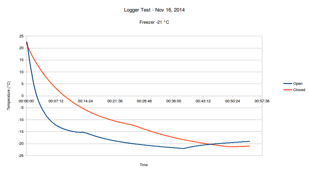
I tested the temperature logger by putting it from room temperature T0 22.6 °C into a freezer at Tm -21.0 °C.

Based on the measurement results below (red graph) it took 54 minutes for the sensor to reach this temperature. The thermal mass of the sensor itself is small, but it was in a closed enclosure with the LiPo battery that has a much larger thermal mass.  I did the same test but this time left the enclosure open so that the sensor was exposed to freezer temperature from both sides.  The blue graph below shows that the sensor reached -21 °C in  30 minutes.

Freezer Test

The thermal time constant is defined as the time required by a sensor to reach 63.2% of a step change in temperature under a specified set of conditions.

The response of a sensor to a sudden change in the surrounding temperature is exponential and it is described by the following equation:

where T is sensor temperature, Tm is the surrounding medium temperature, T0 is the initial sensor temperature, t is the time and τ is the time constant.

Looking at the results above and trying to find best fit of measurement data to this model using RMS error method we can estimate that 

τ  = 0.009732  for closed enclosure

τ  = 0.003132 for open enclosure

See graph of models vs. actuals is below. To correctly estimate temperatures this thermal time constant need to be taken into account.

Model of thermal time constants τ

In the datasheet there are the following guidelines to maintain accuracy.

The temperature sensor in the TMP102 is the chip itself. Thermal paths run through the package leads, as well as the plastic package. The lower thermal

resistance of metal causes the leads to provide the primary thermal path.

To maintain accuracy in applications requiring air or surface temperature measurement, care should be taken to isolate the package and leads from ambient air temperature. A thermally-conductive adhesive is helpful in achieving accurate surface temperature measurement.

One improvement would be to apply thermally-conductive materials between the sensor chip and the bottom surface of the enclosure. Some biologically inert metal like gold or titanium might provide better thermal time constant. Some insulation might be needed to isolate sensor from ambient air. 

Conclusions 

Temperature logging using modern, high resolution and accurate digital sensors is quite easy.  You need only simple a micro-controller and few lines of code to build a data logger that is small enough to be wearable.

Working with Arduinos is not only easy but also a lot of fun.  With minimal investment you can build a powerful data logging device and add new sensors in incremental fashion.  The software development is also straightforward and for most problems there is already some open source examples available.

The real challenges seem to be on the physics and mechanical enclosure design side. Building an enclosure for the sensor and electronics with a small thermal time constant is not trivial.  For highly accurate wearable data logging devices you need also to consider many other topics such as

• physical appearance 
• hypoallergic materials 
• fit and comfort for different size of subjects
• thermal properties of materials
• any variability in sensor contact with subject or ambient air 

It would be interesting to see the thermal design details of popular fitness trackers that claim accurate body temperature measurements. In particular the basal body temperature measurements where accuracy and high resolution is required poor thermal design would impact results significantly.

Morse Learning Machine - Challenge

MACHINE LEARNING CHALLENGE

I was astonished to get email acknowledgement that my  Kaggle Morse Challenge was approved today. I have spent last few days preparing materials and editing the description and the rules for this competition.

The goal of this competition is to build a machine that learns how to decode audio files containing Morse code.

For humans it takes many months effort to learn Morse code and after years of practice the most proficient operators can decode Morse code up to 60 words per minute or even beyond. Humans have also extraordinary ability to quickly adapt to varying conditions, speed and rhythm.

I want to find out if it is possible to create a machine learning algorithm that exceeds human performance and adaptability in Morse decoding.  I have shared some of these ideas in New England Artificial Intelligence meetup about one year ago and got enthusiastic feedback from the participants.

WHY KAGGLE?   

Kaggle is a platform for predictive modelling and analytics competitions on which companies and researchers post their data and statisticians and data miners from all over the world compete to produce the best models. This crowdsourcing approach relies on the fact that there are countless strategies that can be applied to any predictive modelling task and it is impossible to know at the outset which technique or analyst will be most effective. Kaggle aims at making data science a sport.

Kaggle's community of data scientists comprises tens of thousands of PhDs from quantitative fields such as computer science, statistics, econometrics, maths and physics, and industries such as insurance, finance, science, and technology. They come from over 100 countries and 200 universities. In addition to the prize money and data, they use Kaggle to meet, learn, network and collaborate with experts from related fields.

For the Morse Learning Machine competition I hope to attract people from the Kaggle community who are interested in solving new, difficult challenges using their predictive data modeling, computer science and machine learning expertise.  For students this challenge provides a great opportunity to put theoretical concepts into practice and see how they can solve tough problems by applying knowledge gained in class rooms.

COMPETITION DETAILS

During the competition, the participants build a learning system capable of decoding Morse code. To that end, they get development data consisting of 200 .WAV audio files containing short sequences of randomized Morse code. The data labels are provided for a training set so the participants can self-evaluate their systems. To evaluate their progress and compare themselves with others, they can submit their prediction results on-line to get immediate feedback. A real-time leaderboard shows participants their current standing based on their validation set predictions.

I have also provided  sample Python Morse decoder  to make it easier too get started. While this software is purely experimental version it has some features of the FLDIGI Morse decoder   but implemented using Python instead of C++.

You can of course  leverage the experimental multichannel CW decoder I recently implemented on FLDIGI or the standalone version of Bayesian decoder written in C++.  There is also some new tools I posted to Github.

Please help me to spread this message to attract participants for the Morse Learning Machine challenge!

73
Mauri AG1LE

Cortical Learning Algorithm for Morse code - part 1

Cortical Learning Algorithm Overview 

Humans can perform many tasks that computers currently cannot do. For example understanding spoken language in noisy environment, walking down a path in complex terrain or winning in CQWW WPX CW contest are tasks currently not feasible for computers (and might be difficult for humans, too).
Despite decades of machine learning & artificial intelligence research, we have few viable algorithms for achieving human-like performance on a computer. Morse decoding at the best human performance level would be a good target to test these new algorithms.

Numenta Inc.  has developed technology called Cortical Learning Algorithm (CLA) that was recently made available as open source project  NuPIC.  This software provides an online learning system that learns from every data point fed into the system. The CLA is constantly making predictions which are continually verified as more data arrives. As the underlying patterns in the data change the CLA adjusts accordingly. CLA uses Sparse Distributed Representation (SDR) in similar fashion as neocortex in human brain stores information. SDR has many advantages over traditional ways of storing memories, such as ability to associate and retrieve information using noisy data.

Detailed description on how CLA works can be found from this whitepaper.

Experiment 

To learn more how CLA works I decided to start with a very simple experiment.  I created a Python script that uses Morse code book and calculates Sparse Distributed Representation (SDR) for each character.  Figure 1 below shows the Morse alphabet and numbers 0...9 converted to SDRs.

Fig 1. SDR for Morse characters A...Z, 0...9

NuPIC requires input vector to be a binary representation of the input signal.  I created a function that packs "dits" and "dahs" into 36x1  vector, see two examples below. Each "dit"  is represented as 1. followed by 0. and each "dah" is represented by  1. 1. 1. followed by 0.  to accomodate 1:3 timing ratio between "dit" and "dah".  This preserves the semantic structure of Morse code that is important from sequence learning perspective.

H ....
[ 1.  0.  1.  0.  1.  0.  1.  0.  0.  0.  0.  0.  0.  0.  0.  0.  0.  0.
  0.  0.  0.  0.  0.  0.  0.  0.  0.  0.  0.  0.  0.  0.  0.  0.  0.  0.]

O ---

[ 1.  1.  1.  0.  1.  1.  1.  0.  1.  1.  1.  0.  0.  0.  0.  0.  0.  0.

  0.  0.  0.  0.  0.  0.  0.  0.  0.  0.  0.  0.  0.  0.  0.  0.  0.  0.]

The Spatial Pooler uses 64 x 64 vector giving SDR of size 4096. As you calculate the SDR random bits get active on this vector. I plotted all active cells (value = 1) per columns 0...4096 for each letters and numbers as displayed in Fig 1. above. The respective character is shown on the right most column.

To see better the relationships between SDR and Morse character set I created another SDR map with letters  'EISH5' and 'TMO0'  next to each other.  These consequent letters and numbers differ from each other only by one "dit" or one "dah".  See Fig 2.  for SDR visualization of these characters.

There is no obvious visible patterns across these Morse characters, all values look quite different.  In the Numenta CLA whitepaper page 21 it says "Imagine now that the input pattern changes. If only a few input bits change, some columns will receive a few more or a few less inputs in the “on” state, but the set of active columns will not likely change much. Thus similar input patterns (ones that have a significant number of active bits in common) will map to a relatively stable set of active columns."

This doesn't seem to apply in these experiments so I need to investigate this a bit further.

Fig 2. SDR for Morse characters EISH5 and TMO0

I did another experiment by reducing SDR size to only 16x16  so 256 cells per SDR. In Fig 3.  it is now easier to see common patterns between similar characters - for example compare C with K and Y.  These letters have 3 common cells active.

Fig 3. SDR  map with reduced size 16x16 = 256 cells

The Python software to create the SDR pictures is below:

"""A simple program that demonstrates the working of the spatial pooler"""

import numpy as np

from matplotlib import pyplot as plt

from random import randrange, random

from nupic.research.spatial_pooler import SpatialPooler as SP

CODE = {

    ' ': '',

    'A': '.-',

    'B': '-...',

    'C': '-.-.', 

    'D': '-..',

    'E': '.',

    'F': '..-.',

    'G': '--.',    

    'H': '....',

    'I': '..',

    'J': '.---',

    'K': '-.-',

    'L': '.-..',

    'M': '--',

    'N': '-.',

    'O': '---',

    'P': '.--.',

    'Q': '--.-',

    'R': '.-.',

    'S': '...',

    'T': '-',

    'U': '..-',

    'V': '...-',

    'W': '.--',

    'X': '-..-',

    'Y': '-.--',

    'Z': '--..',

    '0': '-----',

    '1': '.----',

    '2': '..---',

    '3': '...--',

    '4': '....-',

    '5': '.....',

    '6': '-....',

    '7': '--...',

    '8': '---..',

    '9': '----.' }

class Morse():

  

  def __init__(self, inputShape, columnDimensions):

    """

     Parameters:

     ----------

     _inputShape : The size of the input. (m,n) will give a size m x n

     _columnDimensions : The size of the 2 dimensional array of columns

     """

    self.inputShape = inputShape

    self.columnDimensions = columnDimensions

    self.inputSize = np.array(inputShape).prod()

    self.columnNumber = np.array(columnDimensions).prod()

    self.inputArray = np.zeros(self.inputSize)

    self.activeArray = np.zeros(self.columnNumber)

    self.sp = SP(self.inputShape, 

self.columnDimensions,

potentialRadius = self.inputSize,

numActiveColumnsPerInhArea = int(0.02*self.columnNumber),

globalInhibition = True,

synPermActiveInc = 0.01

)

    

  def createInputVector(self,elem,chr):

        

    print "\n\nCreating a Morse codebook input vector for character: " + chr + " " + elem

    

    #clear the inputArray to zero before creating a new input vector

    self.inputArray[0:] = 0

    j = 0

    i  = 0

    while j < len(elem) :

      if elem[j] == '.' :

        self.inputArray[i] = 1

        self.inputArray[i+1] = 0

        i = i + 2

      if elem[j] == '-' :

        self.inputArray[i] = 1

        self.inputArray[i+1] = 1

        self.inputArray[i+2] = 1

        self.inputArray[i+3] = 0

        i = i + 4

      j = j + 1

               

    print self.inputArray

     

     

  def createSDRs(self,row,x,y,ch):

    """Run the spatial pooler with the input vector"""

    print "\nComputing the SDR for character: " + ch

    

    #activeArray[column]=1 if column is active after spatial pooling

    self.sp.compute(self.inputArray, True, self.activeArray)

    

    # plot each row above previous one

    z = self.activeArray * row

    # Plot the SDR vectors - these are 4096 columns in the plot, with active cells visible

    plt.plot(x,y,z,'o')

    plt.text(4120,row-0.5,ch,fontsize=14);

    print self.activeArray.nonzero()

    

    

# Testing NuPIC for Morse decoding  

# Create SDRs from Morse Codebook input vectors

print "\n \nCreate SDRs from Morse Codebook input vectors"

# vector size 36x1 for input,  64x64 = 4096 for SDR 

example = Morse((36, 1), (64, 64))

x,y = np.meshgrid(np.linspace(1,1,4096), np.linspace(1,1,32))

plt.ylim([0,38])

plt.xlim([0,4170])

# Select the characters to be converted to SDRs

#str = 'ABCDEFGHIJKLMNOPQRSTUVWXYZ0123456789'

str = 'EISH5 TMO0'

row = 1

for ch in str:

  example.createInputVector(CODE[ch],ch)

  example.createSDRs(row,x,y,ch)

  row = row +1

plt.show()

plt.clf()

Conclusions

CLA provides promising new technology that is now open for ham radio experimenters to start tinkering with. Building a CLA based Morse decoder would be a good performance benchmark for CLA technology. There are plenty of existing Morse decoders available to compare with and it is fairly easy to test decoder accuracy under noisy conditions.  There is also a plenty of audio test material available, including streaming sources like WebSDR stations.

73

Mauri 

New Morse Decoder - part 6

Multichannel CW decoder 

Development of the Bayesian CW decoder is moving forward. Many thanks to Dave W1HKJ  there is now an alpha build available also for Windows platform. The v3.21.83cw-a4  tarball sources and Windows version are available in http://www.w1hkj.com/ag1le/

This version has still multiple problems that need to fixed. In Fig 1. below I have screenshot where I have the multichannel signal browser and Fldigi configuration screen for Modems / CW  visible. I am running Windows FLDIGI version v3.21.83cw-a4  connected to PowerSDR v2.6.4 and my Flex3000 radio.

The following description explains the options and expected behavior in this alpha software version.  Things are not yet  well optimized so you are likely to see a lot of misdecoded signals.  I am interested getting feedback and improvement ideas to make the Bayesian decoder better.

Checkbox "Bayesian decoding" enables multichannel operation. If you have Signal Browser open you can slide the horizontal control at the bottom to adjust the signal decoding threshold. With lower threshold you can enable weaker CW stations to be decoded but often you get just noise and the decoder produces garbage as visible in Fig 1.   The software detects peaks in the spectrum and starts a new decoder instance based on the detected peak signal frequency. It tracks each instance on a channel which is rounded at 100 Hz of the audio signal frequency. Number of channels and timeout value can be set in  Configure/User Interface/Browser menu.

If there are two stations in nearby frequencies less than 20 Hz apart the other one is eliminated.  This is done to reduce impact of frequency splatter - otherwise one strong CW station would spin up decoders on multiple channels. Also, in this version this process is done for every FFT row in the waterfall display. Because I am not doing any kind of averaging yet the detected peak signal center frequency  may be incorrect and therefore decoder is tuned on the wrong frequency. With narrow filter bandwidth setting this may cause garbage in the decoder output.

Fig 1. Multichannel CW decoder 

In this version each decoder instance uses the same filter bandwidth that is set manually in Configure/Modem/CW/General  tab. This means that Bayesian decoder does not have optimal, speed dependent filtering. For faster stations the bandwidth should be larger and for slow stations it can be narrow.
This means that decoding accuracy suffers if there are multiple stations operating at different speeds. Once again this functionality can be improved as the Bayesian decoder does provide a speed estimate automatically but I haven't had time to implement the automatic "Matched filter"  feature yet. The filter bandwidth is taken from the "Filter bandwith" slider value  for all Bayesian  decoder instances.

On receiver speed estimation Rx WPM value is updated only for selected CW signal on the waterfall. You can also observe that with Bayesian decoder enabled the speed display is updated much more frequently than with the legacy CW decoder.  Bayesian decoder calculates speed estimate every 5 msec and provides a WPM value whenever there is a state change  (mark -> space or space->mark) in the signal.  Sometimes the speed estimator gets "stuck" in lower or upper extreme.  You can adjust the "Lower limit" or "Upper Limit" on the CW / General  Transmit  section - this will give a hint to the speed estimator to re-evaluate speed.  Obviously, if the speed estimate is incorrect you will get a lot of garbage text  out from the decoder.

Tracking feature is not implemented properly yet for the Bayesian decoder. This means that if you start to transmit  your speed may be different than the station that you were listening. TX WPM is visible in the configuration screen.

Once again,  this is an alpha release  provided in order to get some feedback and improvement ideas  from FLDIGI users.  You can provide feedback by submitting comments below or sending me email to  ag1le at innomore dot com.   It would be very helpful  if you could provide audio samples (WAV files can be recorded   using File / Audio / RX Capture feature of FLDIGI),  screenshot of what CW parameter settings you are using  and general description of the problem or issue you discovered.

If you are interested in software development I would be very grateful  to get some additional help. Building a Bayesian Morse decoder has been a great learning experience in signal processing, machine learning algorithms  and probability theory.  There are plenty of problems to solve in this space as we  build  more intelligent software to use Morse code, the international language of hams.  

73
Mauri AG1LE

New Morse Decoder - part 5

Multichannel CW decoder for FLDIGI

I have been working on the Bayesian Morse decoder for a while.  The latest effort was focused on making it possible to automatically detect all CW signals in the audio band and spin up a new instance of the Bayesian decoder for each detected signal.

Figure 1. shows a running version implemented on top of FLDIGI  version 3.21.77.  The waterfall shows 9 CW signals from 400Hz to 1200 Hz. The software utilizes the FLDIGI Signal Browser user interface and you can set the signal threshold using the slider bar below the signal browser window. The user interface works very much like the PSK or RTTY browser.

Figure 1. Multichannel CW decoder for FLDIGI

The audio file in this demo was created using Octave script  below

Fs = 8000; % Fs is sampling frequency - 8 Khz
Ts = 10*Fs; % Total sample time is 10 seconds


% create 9 different parallel morse sessions - 10 seconds each at 20-35 WPM speed
%         TEXT           audio file  noiselevel Hz    speed WPM 
x1=morse('CQ TEST DE AG1LE','cw1.wav', 20,1200,Fs,20, Ts);
x2=morse('TEST DE SP3RQ CQ','cw2.wav', 15, 1100,Fs,35, Ts);
x3=morse('DE W3RQS CQ TEST','cw3.wav', 20,  1000,Fs,30, Ts);
x4=morse('SM0LXW CQ TEST DE','cw4.wav',15,   900,Fs, 25, Ts);
x5=morse('CQ TEST DE HS1DX','cw5.wav', 20,    800,Fs, 20, Ts);
x6=morse('TEST DE JA1DX CQ','cw6.wav', 10,      700,Fs, 20, Ts);
x7=morse('DE JA2ATA CQ TEST','cw7.wav',20,      600,Fs, 20, Ts);
x8=morse('UA2HH CQ TEST DE','cw8.wav', 15,      500,Fs, 20, Ts);
x9=morse('CQ TEST DE CT1CX','cw9.wav', 20,      400,Fs, 20, Ts);


% weighted sum - merge all the audio streams together 
% 9 signals arranged in frequency order 1200Hz ... 400Hz
y = 0.1*x1 + 0.1*x2 + 0.1*x3 + 0.1*x4 + 0.1*x5 + 0.1*x6 + 0.1*x7 + 0.1*x8 + 0.1*x9;


% write to cwcombo.wav file 
wavwrite(y,Fs,'cwcombo.wav');

I have saved the full sources of this experimental FLDIGI version in Github:  FLDIGI source
UPDATE July 20, 2014: I rebased this using Source Forge latest branch  - new version is here: fldigi-3.22.0CN.tar.gz

Let me know if you are interested in testing this software.  I would be interested in getting feedback on scalability, any performance problems as well as how well the CW decoder works with real life signals.

73
Mauri AG1LE