Creating Training Material for Recurrent Neural Networks

INTRODUCTION

In my previous post I shared an experiment I did using Recurrent Neural Network (RNN) software.  I started thinking that perhaps RNNs could learn not just the QSO language concepts but also learn how to decode Morse code from noisy signals. Since I was able to demonstrate learning of the syntax, structure and commonly used phrases in QSOs just in 50 epochs after going through the training material, wouldn't the same concept work for actual Morse signals?

Well, I don't really have any suitable training materials to test this. For the Kaggle competitions (MLMv1, MLMv2) I created a lot of training materials but the focus of these materials was different. The audio files and corresponding transcript files were open ended as I didn't want to narrow down possible approaches that participants might take. The materials were designed for a Kaggle competition in mind to be able to score participants' solutions.

In machine learning you typically have training & validation material that has many different dimensions  and a target variable (or variables) you are trying to model. With neural networks you can train the network to look patterns in the input(s) and set outputs to target values when the input pattern is detected. With RNNs you can introduce memory function - this is necessary because you need to remember signal values from the past to properly decode the Morse characters.

In Morse code you typically have just one signal variable and goal is to extract decoded message from that signal. This could be done by having for example 26 outputs for each alphabet character and train the network to set output 'A' to high when pattern '.-' is detected in the signal input. Alternatively you could have output lines for symbols like 'dit' and 'dah' and 'element space' that are set high when corresponding pattern is detected in the input signal.

Since a well working Morse decoder has to deal with different speeds (typically 5 ... 50 WPM), signals containing noise and QSB fading and other factors I decided to create a Morse Encoder software that creates artificial training signals, but also corresponding symbols, speed information etc. I chose to use this symbols approach because it easier to debug errors and problems when you can plot the inputs vs. outputs graphically. See this Wikipedia article for details about representation, timing of symbols and speed.

The Morse Encoder generates a set of time synchronized signals and has also capability to add QSB type fading effects and Gaussian noise. See example of 'QUICK BROWN FOX JUMPED OVER THE LAZY FOX ' plotted with deep  QSB fading with 4 second cycle time and  0.01 sigma Gaussian noise added in Figure 1. below.

Fig 1. Morse Encoder output signal with QSB and noise

The QSB for real life signals doesn't always follow sin() curve like in Fig 1. but as you can see from example below this is close enough. The big challenge is how to continue decoding correctly when the signal goes down to noise level as shown between 12000 to 14000 time samples (horizontal axis) below.

TRAINING MATERIALS

To provide proper target values for RNN training the Morse Encoder creates a Python DataFrame with the following columns defined

    P.t    # keep time  
    P.sig  # signal stored here
    P.dit  # probability of 'dit' stored here
    P.dah  # probability of 'dah' stored here
    P.ele  # probability of 'element space' stored here
    P.chr  # probability of 'character space' stored here
    P.wrd  # probability of 'word space' stored here
    P.spd  # WPM speed stored here 

Using these columns Morse Encoder takes the given text and parameters and then generates values to these columns. For example when there is a 'dit' in the signal, on corresponding rows the P.dit has probability of 1.0. Likewise, if there is a 'dah' in the signal, on corresponding rows the P.dah has probability of 1.0. This is shown on the Figure 2. below - dits are red and dahs are green, while the signal is shown in blue color.

Fig 2.  Dit and Dah probabilities 

Zoomed section of letters 'QUI ' is shown on Fig 3. below.

Fig 3. Zoomed section

Likewise we create probabilities for the spaces. In Figure 4 below element space is shown with magenta and character space with cyan color. I decided to set character space to probability 1.0 only after element space has passed, as can be seen from the graph.

Fig 4. Element Space and Character Space 

The resulting DataFrame can be saved into a CSV file with a simple Python command and it is very easy to manipulate or plot graphs. Conceptually it is like an Excel spreadsheet - see below:

	t	sig	dit	dah	ele	chr	wrd	spd
0	0.000	0.573355	0	1	0	0	0	40
1	0.001	0.531865	0	1	0	0	0	40
2	0.002	0.554412	0	1	0	0	0	40
3	0.003	0.551539	0	1	0	0	0	40
4	0.004	0.536430	0	1	0	0	0	40
5	0.005	0.561438	0	1	0	0	0	40
6	0.006	0.561170	0	1	0	0	0	40
7	0.007	0.546326	0	1	0	0	0	40
8	0.008	0.562902	0	1	0	0	0	40
9	0.009	0.533140	0	1	0	0	0	40

The Morse Encoder software is stored in Github MorseEncoder.py and it is open source.

NEXT STEPS

Now that I have the capability to create proper training material automatically with some parameters, like speed (WPM), fading (QSB) and noise level (sigma) it is a trivial exercise to produce large quantities of these training files.

My next focus area is to learn more about Recurrent Neural Networks (especially LSTM variants) and experiment with different network configurations. The goal would be to find a RNN configuration that is able to learn how to model the symbols correctly, even in presence of noise and QSB or at different speeds.

73
AG1LE

Your next QSO partner - Artificial Intelligence by Recurrent Neural Network?

INTRODUCTION

Few months ago Andrej Karpathy wrote a great blog post about recurrent neural networks. He explained how these networks work and implemented a character-level RNN language model which learns to generate Paul Graham essays, Shakespeare works, Wikipedia articles, LaTeX articles and even C++ code of Linux kernel. He also released the code of this RNN network on Github.

It has been a while since I have experimented with RNNs. At the time I found RNNs difficult to train and did not pursue any further.  Well,  all that has changed in the last year or so. I installed  Andrej's char-rnn package from Github in less than 10 minutes on my Linux laptop using instructions on the Readme.md file. I tested the installation by training the RNN with the Shakespeare's collected texts provided as part of the package.

If you have GPU graphics card (like NVIDIA Titan) the training goes much faster. I did not have this so I let the training run in the background for over 24 hours on my Lenovo X301 laptop . Looking the results the RNN indeed learned to output Shakespeare like language as Andrej explains in his blog post. It certainly took me more than 24 hours to learn English language and I never learned to write dialogue like Shakespeare. Please note that RNN was a "tabula rasa" so it had to learn everything one character at the time - this was pretty amazing result!

I decided to do an experiment to find out if this RNN technology could be used to build a ham radio robot.

TRAINING A HAM RADIO ROBOT

The robot would have to learn how people make CW QSOs in real life. I collected some 10,000 lines of examples of ham radio CW QSOs from various sources. Some examples were complete QSOs, some were short contest style exchanges and some just calling CQ. The quality of the language model depends on the amount of examples in the training file.

To do this properly I would need at least a few megabytes of examples, but I found only about 200 kBytes after a few minutes of Internet search. I copied this material into a single file named "input.txt" in data/QSOs directory and started the training with the following command:

th train.lua  -data_dir "data/QSOs" -gpuid -1  

RNN reads the input data, builds a dictionary, configures the neural network and parameters and starts the training. During training the software outputs examples in the cv directory. This allows you to see how RNN learns from the provided material.

After only 12 epochs  the RNN had already learned some basic concepts like call signs and basic words, but it was not enough training rounds to learn English or proper syntax of CW QSO.

GG3QXP DE WA1AXP/M K

RARR WIS DE M8BPY RR  NAMME FDO RR0S ANOEN CUX/I AO  RNEL SNETSL CL  ATRSO IANLOED UR RV SI MEE DO  RU @  UR RSR IX NUOR IS QS  IN WIEZ DE QEMUM/7 W

After  25 epochs the RNN had reached to the contest section (November Sweepstakes) of the input file. Note that the call signs below (like VE7LP  or K2XC) were not included in the original training file.  RNN has learned the proper call sign syntax from given examples and is generating this text below:

VE7LP 314 Q 52 SK=

K2XC 153 M 68 WNY=

K8CSC 285 A 15 MI=

AE5MX 341 Q 47 SB=

AE7J 419 A 06 WWA=

K5RMC 137 M 43 OK=

KB2QUT 34 U 21 NNY=

K9MIP 120 M 08 WI=

Wow...RNN has also learned November Sweepstakes exchange from provided examples. Even the ARRL sections are correct. Note that RNN is generating these based on learned rules, not just copying provided examples. All this by reading the input text file one character at the time.

After 39 epochs RNN has learned many CW acronyms, RST report and some basic QSO structure, though there is still a lot of nonsense in the output. RNN talks about name, QTH,  weather (WX) and even RIG and antennas:

GUDXTEN/8 IN = NAME HR IS ED ED  QTH IS CHAPOTON FNCI HOO OO DINED MIAD VALT W FO FON CUR DS MS ES TOT FER CL  IW QSO OB ULLOO = QRHPO DE LOOFSD SORK/ISTO= = = RIG HR IS LACKORI WAZH PA WANFOO = WX WR = 2IT WINLE WOOD DES UP 55 FE  HW? + MJ1GJO DE MJ3ASA K
 GUD DX ES 73 G8XFO DE 2E3CUD/9RP @ 
 KC6XQ DE M5WMM/M DE M1TGL/M K
 W63ED DE M5YUE
VVV VVV
CQ CQ CQ DE WA1NX/WA50 WB4AJH/6 KC0AHH K1 WAJH K
WA3JRC DE W4DD/5MM DE KC3GJJ/8 K
 GV8SDE DE 2I8APZ GD ENZ/QRP GD3BOB 
 G1KHC DE G3ECQ/QCP M7Y
VVV VVVVV
CQ CQ CQ DE W3ARJ/0 W11IA DE M9TFO/P WA2MJH/4 K
1BJ0 WA3BH DE MJ1GDS MJ6XW K
 MW6PJP/M DE MW6QIC UR RST HR 459 W QSB M5YES DE 2E6AO QRS 6NT QSO D =  RIG HR IS K70 WNTN = NAME HR IS JIM JEC  QTH IN COLLA NCME HO FEL PU DS MS ES 2INTOOBA MCONTS = = UR RRTR MNNI W IS HOX WBOO ISTEL INYD = =
 GUD RIS HL W0 IN W WOME DEN UTD PO P =

At this point RNN has seen the complete training material only 39 times. It has figured out many rules (like ending its turn on "K") but it has still problems with vocabulary, how to use call signs properly, etc.

After 50 epochs the RNN had already mastered idioms such as TNX FER NICE QSO CU AGN and structure resembles a real QSO:

KC2RD/4 DE W1GJV K
 W1ARD DE KC2RD/3RO UR RST HR 459 W QSB GD3DIA DE GD9GEN @  CD GG2RD/9 DE W1GRV/4 DE GU5TCH/MM R  TNX FER NICE QSO  CU AGN 
M2YXT DE GD5FM UR RST HR 529 W QSB W1GRD DE W1GRR RR  K
GG TI TE UR 33  
IWAMO DE WA6EN 
KC2X DE W1YDH KE9NZE/0 OL  TU 
UR RST HR 309 W QSB = NAME HR IS AANNY WAVEL  FNH COTE TNX QST 
= UR 7S PR = UR RST HR 599 W QSB = HR VY NERVOUS D DE MYUE USD 1S = 
NAME HR IS DI EESTY ==  RIG HR IS HEATH 71 INTO A NME HR IS VILL  HW? 
2E9AAT DE GW6QI UR  TS TAX DEL  NAME H5 UE EU 539 FE KHHJ RS 2E MES LANNY  = 
QRY = NAME HR IS ED ED  QTH IS PARD VORETP

You can also see that some parts (like NAME HR ) are repeating multiple times. This was also noted by Andrej in his experiments. Since the training is done one letter at the time, and not word by word the RNN doesn't really get the context of these phrases.

PRACTICAL APPLICATIONS

This kind of ability to provide predictive text based on language models is widely used in many Internet services. When you type letters into Google search bar it will provide you alternatives based on prediction that has been learned  from many other search phrases. See figure 1 below. 

Figure 1. Predictive search bar

In the same manner  RNN could provide a prediction based on characters entered so far and what it has learned from previous materials. This would be a useful feature for example in a Morse decoder. Also, building a system that would be able to respond semi-intelligently for example in a contest situation seems also feasible based on this experiment.

However, there is a paradigm shift when we start using Machine Learning algorithms. In traditional programming you write a program that uses input data to come up with output data.  In Machine Learning you provide both input data and output data and computer creates a program (aka model) that is then used to make predictions.  See figure 2. below to illustrate this.

Figure 2. Machine Learning paradigm shift

To build a ham radio robot we need to start by defining the input data and expected output data. Then we need to collect large amount of examples that will then be used to train the model. Once the model is able to accurately predict correct output you can then embed it into the overall system. Some systems will continuously learn and update the model on the fly.

In the case of ham radio robot we could focus on automating contest QSOs since the structure and syntax is well defined. In the experiment above RNN learned the rules by seeing the examples only 25 times.  So the system could be monitoring a frequency, perhaps  sending CQ TEST DE <MYCALL> or something similar.  Once it receives a response  it would then generate the output using the learned rules and would wait for acknowledgement and log a QSO.

If the training material covers enough "real life" cases, such as missed letters in call signs, out of sequence replies, non-standard responses etc. the ham radio robot would learn to act like human operator and quickly resolve the issue. No extra programming needed, just enough training material to cover these cases.

CONCLUSIONS

Recurrent Neural Network (RNN) is a powerful technology to learn sequences and to build complex language models.  A simple 100+ line program is able to learn complex rules and syntax of ham radio QSOs in less than 50 epochs when presented only a small number of examples ( < 200 kBytes of text).

Building a ham radio robot to operate a contest station seems to be within reach using normal computers.  The missing piece is to have enough real world training material and to figure out an optimal neural network configuration to learn how to work with human CW operators.  With the recent advances of deep learning and RNNs this seems an easier problem than for example trying to build an automatic speech recognition system.

Happiness Formula

Many people have tried to express human happiness in a mathematical formula. One of my personal favorites is created by Scott Adams (Dilbert fame). However, after many deep thoughts and a few drinks with my buddies I have concluded that Scott did not get the formula quite correct.

The correct and official Happiness Formula is shown in Figure 1. below

Fig 1. Happiness Formula

While Scott tried to explain happiness as a linear combination of each component he missed a few important points.

Integral over time  - human happiness varies over time. Happiness is a fragile mental state that can easily go up or down. True happiness must be an integral over the observation time period.  The time period could be one fantastic night out with good friends celebrating your promotion or over several months when you are fighting for your life in a cancer treatment center. It could also be over a lifetime when you are on your death bed thinking of your life and all the happy experiences. It can also be over the time period when you fell madly in love, got married  and eventually divorced. When you select a different time horizon, you end up with a different happiness value.

Normalization  - to be able to measure happiness you need to normalize the value by dividing the sum of components with expectations. If you expect the world you might not be happy even with the greatest partner or having billion dollars in your pocket. Your happiness depends on your expectations; winning a million dollars in a lottery when you least expect will boost your happiness for a while. If you expect to win 2 millions but you only get 1 million you will be disappointed. A small kid visiting DisneyWorld for the first time is super happy about the experience; an adult visiting same place for the 5th time gets easily bored and is not very happy.

Individual Coefficient - Ci also known as "Ida's constant" by the Finnish waitress who validated Happiness Formula after our happy group had spent significant effort and had many drinks to formulate happiness. This coefficient scales the happiness value for each individual to comply with International Unit of Happiness, aka  "Anand".

Standardized Unit  -  Anand ( आनन्द ) is a Hindi word for happiness.  One Anand is the unit of happiness, much like Tesla is the unit of magnetic flux density.

So there you have it, a mathematically rigorous formula of Happiness.

In the next post we focus on measurement techniques of Happiness and how to calibrate your measurement system against the International Anand standard held in safety in our Boston based laboratory.

Until next time.

Mauri

Internet of Things (IoT) - hype vs. reality

Over the last few years the hype around "Internet of Things" (IoT) has been growing rapidly. According to Gartner Hype Cycle 2015 IoT is peaking currently. Assuming IoT follows this cycle this would mean that we are at the peak of inflated expectations and heading towards the through of disillusionment. See figure 1. below to see how IoT concept is tracking on the hype cycle.

Fig 1. "Peak of Expected Inflated Expectations"

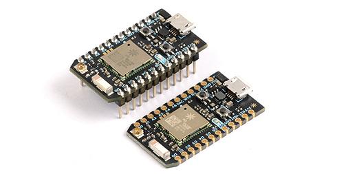
I wanted to learn more about the IoT technology and do some concrete experiments to better understand what IoT can offer. I found the Particle Photon board that is a small $19 Arduino compatible U.S. quarter size board with WiFi enabled Internet connectivity very suitable for prototyping some IoT ideas.  See fig 2. below to get a sense of the size of this tiny board. I ordered two of these just to play a bit and try to build something useful out of these.

Fig 2. Particle Photon board with and without breadboard headers

HUMIDITY CONTROLLER EXPERIMENT

I  already have some previous experience working with Arduino compatible boards such as Arduino Pro Mini that is physically almost the same size of Particle Photon.  In fact I used that board to build a simple humidity controller in our bathroom. This was a quick weekend project where I prototyped on a breadboard a simple circuit with a humidity sensor, a LED indicator and a relay driver to turn the bathroom fan on and off.  I assembled the prototype parts including the breadboard, sensor, relay unit and 12v/5V power supply inside an Apple mouse plastic enclosure. See Fig 3.

Fig 3.  Arduino based humidity controller prototype.

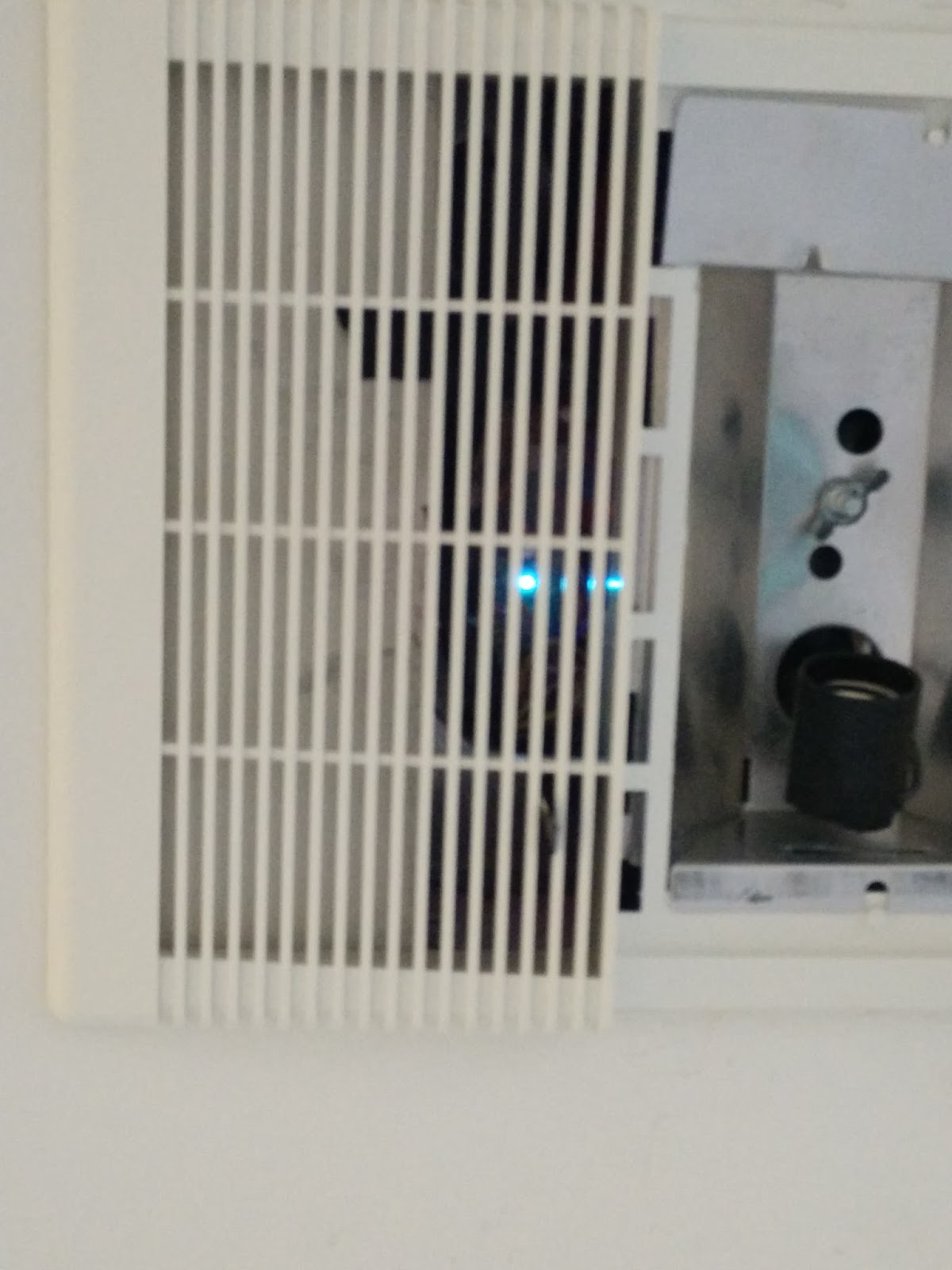
With a few holes drilled on this plastic enclosure to allow air to flow over the sensor I was able to fit the whole controller inside an existing vent box, see Fig 4. below.

Fig 4.  Humidity controller installed inside the vent box.

However,  I did have a problem with this simple controller.  The few lines of software that I wrote in winter time when relative humidity is normally quite low worked very well for many months but during summer months when relative humidity is much higher the software didn't work that well. Debugging this kind of embedded software is not that easy.  I disassembled the prototype for 3 times uploading yet another software version but the damn thing kept starting the vent fan in the middle of night or at some random time.

INTERNET ENABLED HUMIDITY CONTROLLER 

I had to find a solution to this problem so when I learned about the Particle Photon board I knew that this might  just be the solution.  After reading some of the documentation I was pretty sure that having Internet connection would not only help me to debug the problem but also saves me a lot of trouble, as Particle Photon allows you to install the new firmware over the air.  So I wouldn't have the get the vent box  open, remove all wires,  flash the Arduino board with new software and assemble everything back together.

After connecting the Particle Photon board to my Wifi and adding the device on Particle.io web IDE, I used Particle.io web based software development environment (see Fig 5. below) to edit and debug the humidity controller software. I could just simply edit, compile new code, press a button and install firmware almost instantly over the Internet using the WiFi connection on this Photon board.

How cool is this?

Fig 5. Web based software development environment

Particle.io provides also excellent API that have simple to use Internet enabled functions that you can incorporate in your own software. In my case I wanted to debug how the humidity sensor behaves when you have a transient increase in relative humidity when taking a shower.  I used the HTU21D sensor from  Sparkfun. Easy way to debug is to publish your sensor data to the Internet using a simple function like  Spark.publish("RH_temp",str,60,PRIVATE); 

You can use the Particle Dashboard to view the sensor data in near real time. This was almost too easy to describe on a blog like this.

Fig 6. Particle Dashboard

You can use of course use your own web or mobile applications to read and write data as well as control the input/output pins on the Photon board.

I used a simple API command line call to capture the sensor data for plotting:

curl -k https://api.particle.io/v1/devices/<your device id>\/events/?access_token\=<your access token>   >photon_data.txt

Figure 7. below shows the relative humidity transient after taking a shower and then the decline as the vent fan is running.  You can also see the small temperature increase when the hot water is running. When looking at the data I realized that my RH% threshold had been too small. When I increased the threshold value the controller started working much better.  Being able to extract the sensor data and publish it over the Internet made a big difference in debugging the original problem.

Fig 7.  RH% delta and Temperature over time

 

PLOTTING 

In order to collect more data and have a dashboard to plot and review the measurements I signed up for a free account at ThingSpeak. You get an API key and channel number. With these you can plot the values with a simple API call:
ThingSpeak.writeFields(myChannelNumber, myWriteAPIKey);

 Fig 7 and 8 below show the sensor data plot. Relative humidity peaks at 100%  when taking a shower but since the fan is turned on almost instantly the humidity starts to drop quickly back to normal. You can see also a small increase in temperature at the same time. The drop in temperature is due to A/C that turns on at 6:00 AM.

Fig 7. Relative Humidity plot showing a peak

Fig 8. Temperature plot

 

 

 

 

 

 

 

 

 

 

 

 

 

 

 

 

CONCLUSIONS 

My quick foray into the world of "Internet of Things"  took me about 2 hours on a Sunday afternoon. Using the latest  Particle.io Photon board and the web based IDE  I was able to convert my existing Arduino based humidity controller to an Internet enabled controller that is publishing sensor data in near real time and allows me to update the software over the air.

This whole project felt like too easy - I expected that building IoT prototypes would be much harder but at least for this simple use case it took a novice like myself only a short time to solve a real world problem.  Now the bathroom vent works as expected and humidity is under control.

APPENDIX - SOFTWARE 

The current software version is listed below.  As you can see this is not rocket science - a few lines of code and you have an Internet connected sensor / controller.

// This #include statement was automatically added by the Particle IDE.
#include "HTU21D/HTU21D.h"
#include "application.h"
/* 
 HTU21D Humidity Controller
 By: Mauri Niininen (c) Innomore LLC
 Date: Aug 30, 2015


 Uses the HTU21D library to control humidity using a fan.

 Hardware Connections (Breakout board to Photon)
 -VIN = 5.3 V
 -VCC = 3.3 V
 -GND = GND
 -SDA = D0 (use inline 330 ohm resistor if your board is 5V)
 -SCL = D1 (use inline 330 ohm resistor if your board is 5V)

 -RLY = D3   relay board 
 */



#define HOUR  3600/10   // 1 HOUR in seconds - divide by loop delay 10 secs
#define HRS_24 24    // 24 hours of history 

// define class for 24 hr relative humidity 
class RH24 {
private:
  float rh24[HRS_24];  // Keep last 24 hours of humidity 
  int counter;
  int index; 
public:
  void init(float RH);
  void update_h(float RH);  
  float avg(float RH);
};

//Create an instance of the objects
HTU21D mh;
RH24  rh; 

// for time sync
#define ONE_DAY_MILLIS (24 * 60 * 60 * 1000)
unsigned long lastSync = millis();


void setup()
{
  
  
  pinMode(D7, OUTPUT);
  pinMode(D3, OUTPUT);
  
  while (! mh.begin()){
      digitalWrite(D7,HIGH);
      delay(200);
      digitalWrite(D7,LOW);
      delay(200);
  }


  // turn on the fan
  digitalWrite(D3,HIGH);

  // initialize sensor 
  rh.init(mh.readHumidity());  
  delay(5000);
  
  // turn off the fan
  digitalWrite(D3,LOW);
}


// MAIN PROGRAM LOOP 
void loop()
{
  // read sensor humidity and temperature 
  float humd = mh.readHumidity();
  float temp = mh.readTemperature();
  float avg = rh.avg(humd);
  float delta = humd - avg;
  
  // convert data to string
  String h_str = String(humd,2);
  String t_str = String(temp,2);
  String d_str = String(delta,2);
  String avg_str = String(avg,2);
  String tm_str = String(millis());
  String str = String(h_str+":"+t_str+":"+d_str+":"+avg_str+":"+tm_str);
  

  // if relative humidity increases over 12% vs. 24 hour average, turn on the fan 
  if (humd - avg > 12.0) {
    digitalWrite(D7,HIGH);
    digitalWrite(D3,HIGH);
    Spark.publish("RH_temp","ON",60,PRIVATE);
  }
  else {
    digitalWrite(D7,LOW);
    digitalWrite(D3,LOW);
  }


  // time sync over Internet once a day
  if (millis() - lastSync > ONE_DAY_MILLIS) {
    // Request time synchronization from the Particle Cloud
    Spark.syncTime();
    lastSync = millis();
  }
    
  // Send a published string to your devices...
  Spark.publish("RH_temp",str,60,PRIVATE);
  delay(10000);

}


void RH24::init(float RH){
    counter = 0;
    index = 0;
    for (int i = 0; i < HRS_24; i++)
      rh24[i] = RH;
}

void RH24::update_h(float RH) {
    counter += 1;
    if (counter > HOUR) {
      counter = 0; 
      rh24[index] = RH; 
      index += 1;
      if (index >=HRS_24) 
        index = 0;
    }
}  
    
float RH24::avg(float RH) {
    update_h(RH);
    float sum = 0.0;
    for (int i = 0; i < HRS_24; i++)
      sum += rh24[i];
    return (sum/HRS_24);
}

El-bug: a novel Morse decoder based on cockroach neural circuits

April 1, 2015

I have been working on a project to harness the power of biological neural circuits into a practical novel solution for digital communications. I decided to call this project "El-bug" as my focus was to find out how fast biological neural circuits can learn to decode Morse code.

Biological neural circuits have some amazing properties compared to computer based artificial neural networks. State of the art deep learning algorithms require millions of data points and hours or days of repetitions to learn patterns in the data, where as biological neural circuits can often learn new patterns using only a few examples and in time scale of tens of milliseconds. Based on literature biological neural circuits are also adaptive and work well under noisy real world signals.

Computer based learning algorithms require expensive hardware to store gigabytes of training data, GPUs to accelerate the learning process and complicated electronics to convert real world signals into digital pictures, audio or other representations. In comparison biological neural circuits are very small, typically come pre-integrated with sensory organs and require very little power in form of cheap organic energy sources such as glucose.

The hardware used in this project is based on Arduino and the components are available at less than $50 from multiple sources online. The biological neural circuits of American cockroach (Periplaneta americana) is used to power the computation. These fascinating insects are readily available from many sources at low cost,  or sometimes even free of charge.

SYSTEM ARCHITECTURE 

The overall system architecture is shown in Figure 1 below. Arduino Pro Mini (3.3 V/8 MHz) has analog and digital interfaces and it is connected to a RFDuino Bluetooth module. Interface to cockroach neural circuitry is done using analog amplifier with frequency response designed for capturing bio-electrical neural spike signals.  Digital output lines are used to provide electrical stimulation of the nerves.

Figure 1.  El-bug Morse decoder system architecture

COCKROACH ANATOMY AND NEURAL CIRCUITRY

There is a surprising amount of research available on the neural circuitry of Periplaneta americana. For example this source explains:
"The anatomy of the cockroach is exceptionally accessible to electrophysiological experimentation for a variety of reasons. First, from the dorsal, or top, view the cockroach has a distinctive prothorax (the section directly behind, and shielding the head) and wings that give the cockroach its distinctive armored look. When flipped on its back, the ventral aspect of the cockroach reveals the basic segmented body sections distinctive of insects: the head, thorax, abdomen, and legs." 

 See Figure 2 for details of cockroach anatomical features.

Figure 2.  Cockroach Anatomy

After studying possible circuits to utilize I decided to focus on "escaping behavior"  that the common cockroach (Periplaneta americana) exhibits.  This is a  robust behavior of turning away from wind puffs (Camhi et al. 1978). This behavior is termed “escaping behavior” since it is the initial movement when escaping from predators.  This source explains the detailed mechanism and neural circuitry in use:
"Understanding the anatomy of the cockroach nervous system is helpful when examining this escape behavior. The ventral nerve cord (VNC) of the cockroach is along its underbelly, rather than the dorsal side where the nerve cord of most vertebrates is located. The VNC is composed of several giant interneurons (GIs) and at the terminal ganglion afferents project to the dendrites of these GIs.
To detect wind directions, the cockroach has two cerci that are covered by numerous filiform hairs located at the rear of its body (Figure 1). Mechanoreceptors are attached at the base of the filiform hairs and are sensitive to wind puffs. Afferents send the neural signal from the mechanoreceptors to the terminal ganglion and thus provide input to the GIs. Due to its specific location and orientation on the cerci, each mechanoreceptor is sensitive to wind puffs from a specific direction relative to the cockroach. Afferents that are sensitive to similar wind directions are located close to each other within the abdominal ganglion."  Figure 3. from the same source shows typical measurement results as explained in the experiment.

Figure 3. Typical afferent response 

The Arduino Pro Mini provides a low cost circuitry to measure the neural responses and it has 4 analog to digital channels readily available.  An analog  pre-amplifier  such as in Spikerbox can easily produce voltage levels required by Arduino ADC. This is a 10 bit ADC and provides  3.2 mV resolution.  According to this source a single ADC read takes about 100 microseconds that is adequate speed for this purpose.  The goal here is to try to establish a clear differentiation between responses to two types of electrical stimulation, similar to [Yu-Wei 2010]  - see Figure 4  as example.

Figure 4. Neural responses to stimulation

MORSE DECODING PROBLEM 

So given above  how could we build a functioning Morse code  decoder  using these key components? The schema is shown in Figure 5.   Using the Bluetooth module we are sending audio containing noisy Morse code audio as streamed data stream to Arduino.  The software in Arduino does very basic signal processing,  calculates the envelope of the audio signal and after low pass filtering generates stimulus signals that are sent using digital output lines to cockroaches that are organized in a 4 level hierarchy corresponding to the alphabet. If numerals would be included we would need a fifth layer.

At each level of the hierarchy  the corresponding cockroach responds to electrical stimulus and  based on a learned reaction will emit either "dit" or "dah" response. These "dit" and "dah" reactions are collected using the 10 bit ADC from 4 analog channels in Arduino and are organized as a sequence.  Once the complete character has been received a simple "best matching unit"  lookup is performed by Arduino and corresponding matched letter  is sent using the serial interface over Bluetooth.

Implementing this scheme in Arduino Pro Mini did take some effort as available RAM memory is only 2 kilobytes.  After about 2 weeks of coding effort I managed to squeeze all the functionality in and have still some 343 bytes of RAM free.

Figure 5.  Morse decoding schema using cockroach hierarchy

EXPERIMENTAL  RESULTS 

I did run a 20 hours of tests using El-bug Morse decoder. I compared the character error rate (CER) to signal to noise ratio (SNR) of the audio files with the previous results achieved using Bayesian Morse decoder. The results are shown in Figure 6 below.   I had to stop the experiment after 20 hours as  2 of the 4 cockroaches got tired of constant stimulation. They seem to have maximum decoding rate of 100 words per minute.

Surprisingly the decoding accuracy of El-bug system appears to to be quite a lot of better compared to my previous records.  With decent signal to noise ratio (> 12 dB @500Hz)  the decoding accuracy approaches 99%.  Even at lower SNR values  El-bug outperforms any known machine learning algorithms that I have tested so far.

Figure 6.  Experimental CER vs. SNR results 

For the next version I am looking into integrating the electronic circuitry into a smaller form factor, something similar to Figure 7. below.  This source provides additional inspiration to pursue this project further.

Figure 7.  Portable El-bug Morse Decoder 

CONCLUSIONS 

If the reader has had patience to follow this story this far I must congratulate you.  You have amazing neural circuitry in your brain  that is able to absorb this amount of information and form an opinion about what is being presented to you.  You may have already realized that this story may be just pure imagination and has no connection to reality whatsoever.


Happy April 1, 2015!

Mauri  AG1LE