Raspberry Pi: APRS tracker mash-up

I wanted to test how Raspberry Pi would work as a small web server  so I installed NGINX  and configured it using the instructions in here. 

I also created a small Javascript page that uses  aprs.fi  JSON API  and Nokia Maps API to track  APRS enabled station on a map.  The source code is posted in github  - this is basically just one file 'index.html'  that is copied to /var/www directory on Raspberry PI.   You need to get the APRS.FI API key from  here.

Here is how the page looks like as served by Raspberry Pi  - see W1MRA-C station  near Prudential Center in Boston.  As you can see from the source code this is a very simplistic Javascript mash-up. 


However, Nokia Maps APIs  do provide a rich set of functionality that can be used to extend the capabilities.  The neat thing here  is that even a tiny web server like Raspberry Pi  can provide this rich functionality because all the heavy lifting is done by Nokia on the maps API side and on the browser doing the page rendering.  

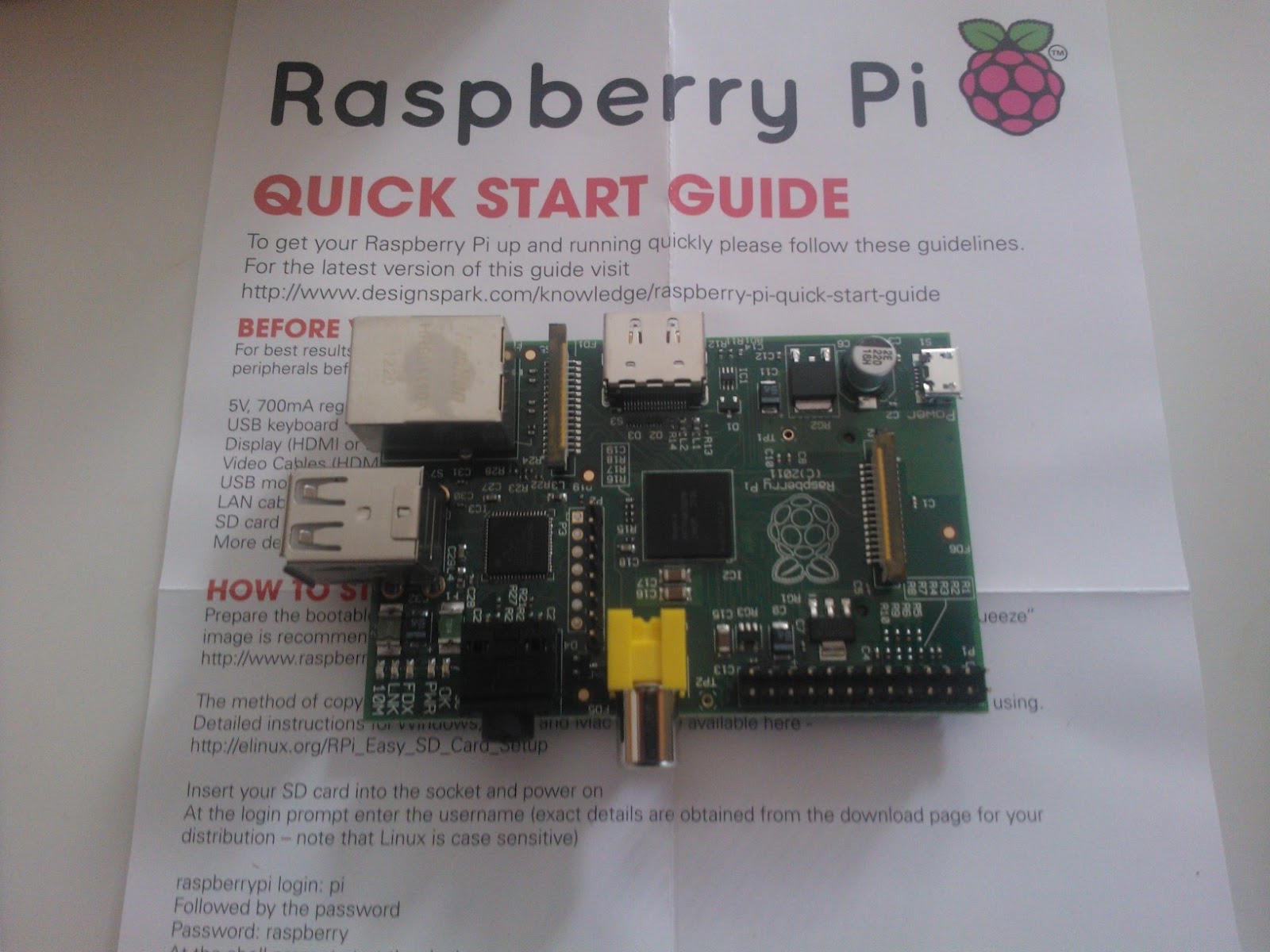
Raspberry Pi Arrived!

I placed the Raspberry Pi order to RS Components  in early March and this credit card sized  $35  Linux computer finally arrived on Monday.  

I created a new page for Raspberry Pi related projects and experiments. Please check in here.  

Morse code detection using modified Morlet Wavelet transformation

In my previous blog post I shared some experiments with wavelets using available online tools.  In order to build better understanding on how to apply Morlet wavelets in detecting Morse code in noisy signals I wrote a little test application using Octave.   The application creates noisy Morse code and does Continuous Wavelet Transform (CWT) using modified Morlet  wavelet as well as Short Term Fourier Transform (STFT).  The Octave application allows changing various parameters and visualizing the impact on the plotted graphs and images.  See discussion on modification to Morlet wavelet below. 

The starting point was original noisy Morse code signal  that has -12.2 dB SNR as shown in the figure 1 below.  It is virtually impossible to detect the Morse signal buried in the noise. When listening the audio I can hear a faint sound in the noise but I have much difficulties recognizing any of the characters.
  
For reference, the signal-to-noise ratio calculation is done the following way: 

SNR=20*log10(norm(morsecode)/norm(morsecode-noisey_morsecode));

Figure 1.   Morse code with -12.2 dB SNR (signal-to-noise ratio)

To discover the Morse code signal I used Short Time Fourier Transformation (STFT)  with the following parameters ( x contains noisy audio,  sampling rate is Fs=4000 )

z = stft(x,1/Fs,4,128,1,512);

A very faint Morse signal is now visible at 600 Hz frequency as a horizontal pattern of "dits and "dahs" in figure 2. below.  It is very difficult to "read" from this figure 3 below what the message is.  Some "dits" and "dahs" are more visible but noise makes it difficult to detect the pattern or to decode the message. 

Figure 2.  Waterfall spectrogram of the Morse code with -12.2dB SNR.

Modified Morlet Wavelet power spectrum is shown on figure 3.  On Scale axis (vertical) you can see  at S = 8 as a horizontal pattern of lighter "dits" and "dahs".  Looking at the pattern you can almost see "dah-dit-dah-dit"  "dah dah dit dah"  "dah dit dit" "dit"  "dit dah" "dah dah dit" "dit dah dah dah dah" "dit dah dit dit"  "dit"   aka  "CQ DE AG1LE".  This represents the peak energy of the power spectrum  after Wavelet transformation. I am taking absolute value to show the envelope of the wavelet better  (see morlet.m file below, calculation is done by this line:    coeffs(k,:)=abs(fftshift(ifft(fft(w).*fft(sigin)))); )

Figure 3.  Wavelet Power Spectrum of the Morse code with -12.2 dB SNR

I plotted Wavelet coefficient C(t,8) values  (corresponding Scale = 8 above) on  x-y graph below in figure 4.  Morse code "dits" and "dahs"  are quite visible as signal peaks above threshold value of 2000.  Note that these are  abs(C(t,8))  values and low pass filtered to show envelope better. See morletdemo.m below for details.

Figure 4.  Modified Morlet coefficient C(8) values.

Original Morlet  wavelets (scales 1 to 16 shown below in figure 5.) have variable wavelet pulse length and frequency as follows: 



for k=1:scale,
    t=(-M/2:M/2-1);
   
    % Calculate Morelet Wavelet w=e-(at^2)*cos(2*pi*fo*t)
    const = 1/(sigma*K*sqrt(k)); % k impacts relative amplitude
    e = exp(-((sigma*t/k).^2));    % k impacts pulse length (t/k)
    phase = cos(2*pi*fo*t/k);    % k impacts frequency 
    w = const*e.*phase;
    plot(w) 
end

While experimenting with these wavelets it was quite difficult find the optimal wavelet to extract signal from noise. 

Figure 5.  Morlet wavelets 1...16

Looking at the impact of various parameters it became obvious that by modifying the wavelet to keep the duration constant improves the situation a lot.  I modified a single line and the corresponding wavelet graph is below in figure 6.   

  e = exp(-((sigma*t).^2));    % removed k to keep the wavelet duration constant.

Note that wavelet bandwidth sigma depends on Morse speed - I did several experiments and established the following relationship  sigma  = (1.2/speed)/w   where w is the number of the wavelet.

Figure 6.   Morlet Wavelet 

CONCLUSIONS 

With a small modification to Morlet wavelet the CWT works better than STFT in extracting the signal from the noise even at -12 dB SNR.  There are many similarities to Matched Filter method that I described in this blog post. Perhaps the main difference is the selected wavelet shape (Morlet) and the fact we use FFT to make the convolution very fast.  

Further work could include the following tasks:

• program  the modified  Morlet Wavelet algorithm in C++ 
• implement this functionality in FLDIGI  CW decoder module
• test Wavelet based decoder with real life signals from HF bands

SOFTWARE 

The Octave scripts are listed below.  The above results were created by running the following command on Octave: 

%  noise level,  signal freq, sampling rate, morsespeed
morletdemo(2,600,4000,20)

The software prints these lines

text = CQ de AG1LE
file = CQ.wav
SNR =-12.226566
Fo =  1.2000
sigma =  0.0075000

and plots the figures.


File Morlet.m


% Project 2
% Time-Frequency Representations
% Andy Doran, modified by  AG1LE Mauri Niininen 
% 
% function coeffs = cwvt(sigin,scale,quiet,sigma,fo)
%
% sigin  = sampled input signal (Should be a row vector)
% scale  = number of real, positive scale you want (1:scales)
% quiet  = plot suppression
%          1 -> suppress all plots
%          2 -> suppress wavelet plots only
%          3 -> suppress scalogram only
% sigma =0.015625;     Morlet Wavelet bandwidth
% fo = 0.25;           Center frequency of Wavelet
% coeffs = scales-by-length(sigin) matrix returning CWT of sigin at
%          each scale from 1 to scale
%
% This function takes an input signal and computes the Continuous Wavelet
% Transform at different scales using a sampled Morlet Wavelet
%
% Morelet Wavelet w(t) = (1/sigma*K)*exp-((sigma*t)^2)*cos(2*pi*fo*t)


function coeffs = morlet(sigin,scale,quiet,sigma,fo)




K = 1;           % Not sure what this is, so set to 1


M = length(sigin);
coeffs = zeros(scale,M);


for k=1:scale,
    t=(-M/2:M/2-1);


    % Calculate Morelet Wavelet w=e-(at^2)*cos(2*pi*fo*t)
    const = 1/(sigma*K*sqrt(k)); % k impacts relative amplitude
    e = exp(-((sigma*t).^2));    % removed k to keep the wavelet duration constant
    phase = cos(2*pi*fo*t/k);    % k impacts frequency 
    w = const*e.*phase;


    % Plot wavelet in time domain and frequency domain
    if ((quiet ~= 1) & (quiet ~= 2))
      figure(3)
      if (k == 1)  % Clear plot on initial run-through
        clf
      end
      subplot(scale,2,(2*k)-1)
      plot(w)
      txt = ['Modified Morlet Wavelet at scale ', num2str(k)];
      title(txt)
      %figure(4)
      %if (k == 1)  % Clear plot on initial run-through
      %  clf
      %end
      subplot(scale,2,2*k)
      plot(abs(fft(w)))
      txt = ['Frequency Spectra of Morlet Wavelet at scale ', num2str(k)];
      title(txt)
   end
    % Calculate CWT of sigin using circular convolution
%    coeffs(k,:)=ifft(fft(w).*fft(sigin));
    coeffs(k,:)=abs(fftshift(ifft(fft(w).*fft(sigin))));
end


% Coeffs should be real anyway, this just accounts for numerical error
% in circular convolution that may give small imaginary parts
coeffs = real(coeffs);


% Plot scalogram and check against MATLAB's CWT routine
if ((quiet ~= 1) & (quiet ~= 3))
  figure(1)
  %clf
  map = jet();
  colormap(map);
  imagesc(coeffs);
  axis xy;
  txt = ['abs|C(t,s)| for s = 1 to ' num2str(scale)];
  title(txt)
  ylabel('s')
  xlabel('t')
  figure(2);
  plot(sigin);  
  title('original signal');
 %figure(4);
  %clf
  %cwt(sigin,1:scale,'morl','plot');  % Call MATLAB's CWT routine
  %title('CWT Output from MATLAB')
end


File  stft.m


function y = STFT(x, sampling_rate, window, window_length, step_dist, padding)
%
%  y = STFT(x, sampling_rate, window, window_length, step_dist, padding)
%
%  STFT produces a TF image of "x".
%  The output is also stored in "y".
%
%  For "window", use one of the following inputs:
%  rectangular    = 1
%  Hamming        = 2
%  Hanning        = 3
%  Blackman-Tukey = 4
%
%  The time scale is associated with the center of the window,
%  if the window is of odd length.  Otherwise, the window_length/2
%  is used.  "Step_dist" determines the stepping distance between the number
%  of samples, and is arranged to maintain the proper time index
%  provided by "sampling_rate" in seconds.  "Padding" is the
%  total length of the windowed signal before the fft, which is
%  accomplished by zero padding.
%
%  Developed by Timothy D. Dorney
%               Rice University
%               April, 1999
%               tdorney@ieee.org
%
%  Coded using MATLAB 5.X.X.
%  See http://www.clear.rice.edu/elec631/Projects99/mit/index2.htm
%
% REVISION HISTORY
%
% VERSION 1.0.0 APR. 21, 1999 TIM DORNEY
%


if (nargin ~= 6)
        disp('STFT requires 6 input arguments!')
return;
end
if ((window < 1) | (window > 4))
window = 1;
disp('The argument "window" must be between 1-4, inclusively.  Window set to 1!');
end
if ((step_dist < 1) | (round(step_dist) ~= step_dist))
step_dist = 1;
disp('The argument "step_dist" must be an integer greater than 0.  Step_dist set to 1!');
end
if (sampling_rate <= 0)
disp('The argument "sampling_rate" must be greater than 0.');
break;
end
if (padding < window_length)
padding = window_length;
disp('The argument "padding" must be non-negative.  Padding set to "window_length"!');
end


if (window == 1)
WIN = ones(1,window_length);
elseif (window == 2)
WIN = hamming(window_length)';
elseif (window == 3)
WIN = hanning(window_length)';
elseif (window == 4)
WIN = blackman(window_length)';
end


[m,n] = size(x);
if (m ~= 1)
X = x';
else
X = x;
end
[m,n] = size(X);
if (m ~= 1)
disp('X must be a vector, not a matrix!');
break;
end


LENX = length(X);
IMGX = ceil(LENX/step_dist);
if (padding/2 == round(padding/2))
IMGY = (padding/2) + 1;
else
IMGY = ceil(padding/2);
end


y = zeros(IMGX,IMGY);


if (window_length/2 == round(window_length/2))
CENTER = window_length/2;
x_pad_st = window_length - CENTER - 1;
x_pad_fi = window_length - CENTER;
else
CENTER = (window_length+1)/2;
x_pad_st = window_length - CENTER;
x_pad_fi = window_length - CENTER;
end


X = [zeros(1,x_pad_st) X zeros(1,x_pad_fi)];


iter = 0;
for kk = 1:step_dist:LENX
iter = iter + 1;
XX = X(kk:(kk + window_length - 1));
YY = XX .* WIN;
ZZ = abs(fft(YY, padding));
y(iter,:) = ZZ(1:IMGY);
end
figure(6);
freq = (1/sampling_rate)/2;
imagesc([0:(step_dist*sampling_rate):(sampling_rate*(LENX-1))], ...
[0:(freq/(IMGY-1)):freq],y');
xlabel('Time (seconds)');
ylabel('Frequency (Hz)');
axis('xy')

File  morletdemo.m


function morletdemo(noisy,freq,Fs,speed);


x = morse('CQ de AG1LE','CQ.wav',noisy,freq,Fs,speed);


w = 8;         %  peak will be at wavelet # w
Fo = freq / (Fs/w)     % tell wavelet transform where wavelet center frequency is 
sigma  = (1.2/speed)/w  % wavelet bandwidth - impacts time resolution


c = morlet(x',16,2,sigma,Fo);         % do Morlet wavelet transform
y = filter(ones(1,20)/20,1,c(w,:));   % y = low pass filter C(t,w) wavelet 
figure(4)
plot(y);                              % plot C(t,w) envelope


z = stft(x,1/Fs,4,128,1,512); % plot spectrogram of the signal using Short Term FFT 
end;




File  morse.m

function code=morse(varargin)

% MORSE converts text to playable morse code in wav format

%

% SYNTAX

% morse(text)

% morse(text,file_name);

% morse(text,file_name,noise_multiplier);

% morse(text, file_name,noise_multiplier,code_frequency);

% morse(text, file_name,noise_multiplier,code_frequency,sample_rate);

% morse(text, file_name,noise_multiplier,code_frequency,sample_rate, code_speed_wpm, zero_fill_to_N);

% morse(text, file_name,noise_multiplier,code_frequency,sample_rate, code_speed_wpm, zero_fill_to_N, play_sound);

%

% Description:

%

%   If the wave file name is specified, then the funtion will output a wav

%   file with that file name.  If only text is specified, then the function

%   will only play the morse code wav file without saving it to a wav file.

%   If a noise multiplier is specified, zero mean addative white Gaussian

%   noise is added with 'amplitude' noise_multiplier.

%

% Examples:

%

%   morse('Hello');

%   morse('How are you doing my friend?','morsecode.wav');

%   morse('How are you doing my friend?','morsecode.wav', 0.01);

%   morse('How are you doing my friend?','morsecode.wav', 0.01, 440, ,20, Fs);

%   x = morse('How are you doing my friend?','morsecode.wav', 0.01, 440, 20, Fs, 2^20,1); %(to play the file, and make the length 2^20)

%

%   Copyright 2005 Fahad Al Mahmood

%   Version: 1.1 $  $Date: 08-Jul-2010

%   Modifications: Rob Frohne, KL7NA

%Defualt values

Fs=48000;

noise_multiplier = 0;

f_code = 375;

code_speed = 20;

text = varargin{1}

if nargin>=2

file = varargin{2}

end

if nargin>=3

noise_multiplier = varargin{3};

end

if nargin>=4

f_code = varargin{4};

end

if nargin>=5

Fs = varargin{5};

end

if nargin>=6

code_speed = varargin{6};

end

if nargin>=7

length_N = varargin{7};

end

if nargin>=8

playsound = varargin{8};

end

t=0:1/Fs:1.2/code_speed; %One dit of time at w wpm is 1.2/w.

t=t';

Dit = sin(2*pi*f_code*t);

ssp = zeros(size(Dit));

#Dah fixed by Zach Swena 

t2=0:1/Fs:3*1.2/code_speed;  # one Dah of time is 3 times  dit time

t2=t2';

Dah = sin(2*pi*f_code*t2);

lsp = zeros(size(Dah));    # changed size argument to function of Dah 

#Dah = [Dit;Dit;Dit];

#lsp = zeros(size([Dit;Dit;Dit]));

% Defining Characters & Numbers

A = [Dit;ssp;Dah];

B = [Dah;ssp;Dit;ssp;Dit;ssp;Dit];

C = [Dah;ssp;Dit;ssp;Dah;ssp;Dit];

D = [Dah;ssp;Dit;ssp;Dit];

E = [Dit];

F = [Dit;ssp;Dit;ssp;Dah;ssp;Dit];

G = [Dah;ssp;Dah;ssp;Dit];

H = [Dit;ssp;Dit;ssp;Dit;ssp;Dit];

I = [Dit;ssp;Dit];

J = [Dit;ssp;Dah;ssp;Dah;ssp;Dah];

K = [Dah;ssp;Dit;ssp;Dah];

L = [Dit;ssp;Dah;ssp;Dit;ssp;Dit];

M = [Dah;ssp;Dah];

N = [Dah;ssp;Dit];

O = [Dah;ssp;Dah;ssp;Dah];

P = [Dit;ssp;Dah;ssp;Dah;ssp;Dit];

Q = [Dah;ssp;Dah;ssp;Dit;ssp;Dah];

R = [Dit;ssp;Dah;ssp;Dit];

S = [Dit;ssp;Dit;ssp;Dit];

T = [Dah];

U = [Dit;ssp;Dit;ssp;Dah];

V = [Dit;ssp;Dit;ssp;Dit;ssp;Dah];

W = [Dit;ssp;Dah;ssp;Dah];

X = [Dah;ssp;Dit;ssp;Dit;ssp;Dah];

Y = [Dah;ssp;Dit;ssp;Dah;ssp;Dah];

Z = [Dah;ssp;Dah;ssp;Dit;ssp;Dit];

period = [Dit;ssp;Dah;ssp;Dit;ssp;Dah;ssp;Dit;ssp;Dah];

comma = [Dah;ssp;Dah;ssp;Dit;ssp;Dit;ssp;Dah;ssp;Dah];

question = [Dit;ssp;Dit;ssp;Dah;ssp;Dah;ssp;Dit;ssp;Dit];

slash_ = [Dah;ssp;Dit;ssp;Dit;ssp;Dah;ssp;Dit];

n1 = [Dit;ssp;Dah;ssp;Dah;ssp;Dah;ssp;Dah];

n2 = [Dit;ssp;Dit;ssp;Dah;ssp;Dah;ssp;Dah];

n3 = [Dit;ssp;Dit;ssp;Dit;ssp;Dah;ssp;Dah];

n4 = [Dit;ssp;Dit;ssp;Dit;ssp;Dit;ssp;Dah];

n5 = [Dit;ssp;Dit;ssp;Dit;ssp;Dit;ssp;Dit];

n6 = [Dah;ssp;Dit;ssp;Dit;ssp;Dit;ssp;Dit];

n7 = [Dah;ssp;Dah;ssp;Dit;ssp;Dit;ssp;Dit];

n8 = [Dah;ssp;Dah;ssp;Dah;ssp;Dit;ssp;Dit];

n9 = [Dah;ssp;Dah;ssp;Dah;ssp;Dah;ssp;Dit];

n0 = [Dah;ssp;Dah;ssp;Dah;ssp;Dah;ssp;Dah];

text = upper(text);

vars ={'period','comma','question','slash_'};

morsecode=[];

for i=1:length(text)

if isvarname(text(i))

morsecode = [morsecode;eval(text(i))];

elseif ismember(text(i),'.,?/')

x = findstr(text(i),'.,?/');

morsecode = [morsecode;eval(vars{x})];

elseif ~isempty(str2num(text(i)))

morsecode = [morsecode;eval(['n' text(i)])];

elseif text(i)==' '

morsecode = [morsecode;ssp;ssp;ssp;ssp];

end

morsecode = [morsecode;lsp];

end

if exist('length_N','var')

append_length = length_N - length(morsecode);

if (append_length < 0)

printf("Length %d isn't large enough for your message; it must be > %d.\n",length_N,length(morsecode));

return;

else

morsecode = [morsecode; zeros(append_length,1)];

end

end

noisey_morsecode = morsecode + noise_multiplier*randn(size(morsecode));

SNR=20*log10(norm(morsecode)/norm(morsecode-noisey_morsecode));

printf('SNR =%f\n',SNR);

if exist('file','var')

wavwrite(noisey_morsecode,Fs,16,file);

if exist('playsound')

system(['aplay ',file]);

end

else

soundsc(noisey_morsecode,Fs);

% wavplay(morsecode);

end

code = noisey_morsecode;

endfunction

Ultimate Morse Code Decoder?

Over the last few weeks I started reading articles and papers about wavelet transformation to figure out how to build an ultimate Morse code decoder. Wavelets have been used since 1980's in digital signal processing and wavelet transforms are now being adopted for a vast number of applications, often replacing the conventional  Fourier transformation.

One particular application is for smoothing/denoising data based on wavelet coefficient thresholding, also called wavelet shrinkage. By adaptively thresholding the wavelet coefficients that correspond to undesired frequency components smoothing and/or denoising operations can be performed.

WAVELETS FOR DETECTING NOISY SIGNALS

I stumbled on this paper from Aly, Omar and Eldherbeni few days ago. The paper describes an algorithm for extracting and localizing an RF radar pulse from a noisy background. The algorithm combines two powerful tools: the wavelet packet analysis and higher-order-statistics (HOS). The use of the proposed technique makes detection and localization of RF radar pulses possible in very low signal-to-noise ratio conditions. 

The proposed algorithm is able to detect and well localize RF radar pulses without a prior knowledge of the pulse parameters (e.g., its frequency and duration). The proposed  algorithm has been tested for SNR down to −24 dB and proved to work successfully. See figures 9 and 7 below on the results they achieved.

In my previous blog post  I used matched filter to extract Morse code pulses from noisy signals. Matched filter can be implemented  either in time or frequency domain. However,  one problem with narrow matched filter is "ringing" artifacts  - see figure 8  in the blog post. This creates uncertainty and jitter in pulse width.  According to above paper  one of the advantages of  using wavelets is possibility to obtain adapted tiling in the time-frequency plane, which is automatically generated based on the signal observation. This leads to improved time & frequency resolution compared to traditional short-time windowed Fast Fourier Transformation (SFFT) based methods.  

DIFFERENT WAVELET TRANSFORMATIONS

I found this website that provides online tools to visualize various wavelet types. Since the discovery of wavelets many years ago there has been active development and many different wavelets have been created for various purposes. This site provide very nice online visualization tool.

I created  a small noisy Morse code file using  morse.m  Octave function by Rob Frohne, KL7NA.  The above website allows only 2000 samples so I copied numbers to the above site (select "Your data" section).
Figures 1..3  below show a small noisy audio section with a "dit" tone  and start of "dah" tone and corresponding wavelet transformation (Morlet, Gaussian & Paul wavelet types) underneath.  There is also a global wavelet showing the variance by period on the right side.  The wavelet transformation values are color coded - red color is showing the highest energy at Period (scale) 8 clearly identifying where the tone starts and where it ends.  Different wavelets have slightly different properties as is quite visible looking at the figures below.

Figure 1.  Morlet Wavelet - noisy Morse code

Figure 2.  Gaussian Wavelet - noisy Morse code

Figure 3.  Paul Wavelet - noisy Morse code

MORLET WAVELET TRANSFORMATIONS 

As the results from previous section demonstrate Morlet type wavelets seem to provide particularly good delineation of Morse code tones in noisy signals.   I did three more visualizations with  various level of noise included in the signals.  The first one (MORSE_SNR0) below has no noise and the signal is visible as clear red color  line on wavelet power spectrum image (period = 8). It is very easy to see where the signal ends and next one starts (see the gap between samples 1450 ...1900 ). 

The following visualization (MORSE_SNR1) has approximately - 9 dB  SNR  and quite a lot of noise. The red line is still visible in the wavelet power spectrum image (period = 8). However,  noise spikes make it a bit more difficult to determine signal end and start timing. There is also other red noise signals at periods 32, 64 and 256. As these are on different wavelet periods they can be filtered out. 

The last visualization (Morse_SNR2)  has  approximately  - 12 dB SNR  and it is quite difficult to see where the tone ends and next one starts. Looking from original signal it is almost impossible to tell where the tone is.  Global wavelet shows a peak at period 8  where most of the red dots are also aligned. There are many more red areas showing noise energy peaks.

WAVELETS FOR PULSE TRAIN

I  did another experiment with Morse code pulse train.  This is the envelope of the noisy audio signal after detection and filtering. Pulse train has some sharp edges that should correspond to high frequency components as well as longer stable plateaus corresponding low frequency components. 

I used  Haar and Gaussian wavelets in this experiment. Figure 4 and 5 below show the signal and corresponding wavelet transformation.  As expected the high frequency components are visible where the signal edges are.

Figure 4. Haar Wavelet - noisy Morse code pulse train

Notice the red high energy components between 600 - 750 ms in scale 128..512 range. This represents noise that is visible also on the time domain signal in figure 5.  In a wavelet filter implementation these  coefficients could be set to zero  to denoise the signal.

Figure 5. Gaussian Wavelet - noisy Morse code pulse train

CONCLUSIONS

Wavelet transformation  is a powerful signal processing tool to manipulate signals. Based on literature the wavelet transform gives better localization in the time-frequency domain than the discrete windowed Fourier transform.  Wavelets enable also flexible manipulation of the signals to remove noise, find signals buried under noise  etc. 

For a real time CW decoding software like in FLDIGI  wavelet transformation could open a whole new performance level dealing with noisy signals.  More experimentation is definitely needed to unlock this potential.


73
Mauri AG1LE

FLDIGI - Analysing SOM decoder errors

In my previous blog post I shared some test results on new alpha version of Fldigi.

The new version of the Fldigi software works pretty well but occasionally it still generates some decoding errors.  I spent some time today in instrumenting the CW.CXX module to collect some measurements during the normal CW decoding operation.

COLLECTING DATA 

The first place to focus was on how the software detects  "dits" and "dahs" from the incoming signal.
The cw::handle_event() function keeps track of CW_KEYDOWN_EVENTs and CW_KEYUP_EVENTs based on signal thresholds in the new  cw::decode_stream() function.
Therefore this was an obvious place to put a hook.  I created a new function cw::histogram() that collects the current duration value after CW_KEYUP_EVENT is detected. I placed the collection after the noise spike code as these values are not collected for decoding anyways.

I recorded about 3:17 into an audio file from 14 Mhz band with multiple CW stations having contacts. The band was quite noisy and I could see some decoder errors on the Fldigi instance I had connected to my Flex3000.  I replayed the processed audio file on Linux environment with instrumented version of Fldigi.  Figure 1 below shows the probability distribution of "dits" and "dahs".  There are multiple peaks visible and I also noticed that automatic Morse speed tracking changed from 16 WPM to  13 WPM, corresponding to "dit" values of 75ms and 92 ms respectively.  There are also a small number of outliers between 100 and 250 ms range.

Figure 1.  Dit & Dah timing distribution.

Since I was using the SOM decoder  for this experiment I decided to utilize a very nice feature built-in to the Best Matching Unit algorithm.  Since we are calculating Euclidian distance between incoming data vectors and codebook weight vectors and selecting the codebook vector with smallest distance we can use this distance as an error metric.  In other words if the best matching unit did not really provide a good match the distance (diffsf variable in the find_winner() function) should be higher than normally.
I  plotted figure 2  in order to demonstrate where SOM decoder indicated it had trouble matching the right codebook entry.  Not surprisingly when looking at each decoded character with high (over 0.05) error metric you can see some problem with the input vector.  The mean error value was 0.0125 and standard deviation was 0.047556. As you can see the the figure 2 the maximum was 0.50672  and there are several other peaks over 0.1 below.   Each entry on x-axis corresponds to one detected character and y axis is the SOM decoder error.

Figure 2.  SOM decoder - errors over time

Since there are so many error peaks in the figure 2  I started wondering if there is something else than just noise peaks that could be causing problems for the SOM decoder.  In most cases where SOM decoder indicates a bad match there was either additional "dit" or "dah" elements concatenated to the input vector  or some values that were not "dit" or "dah"  according to timing distribution shown in figure 1.

I let the voice file play again and plotted two other variables on the same timescale.  Agc_peak is used to determine with the threshold when signal is considered going up or down and it is a variable itself with fast attack and slow decay. If agc_peak falls down that means that signal level is also going down giving an indication on potential signal-to-noise problem.

Cw_adaptive_receive_threshold is a variable tracking the duration of 2 * "dit" length with a time constant defined by trackingfilter. This is a key variable determining whether received key down event was a "dit" or "dah".  If this variable is not able to follow the changing Morse speed then SOM decoder could get incorrectly assigned "dit" and "dah" values in the  input vector.

I normalized these 3 variables to  [0.0 1.0] range and plotted them on the same graph to see if there are any dependencies.  Figure 3  shows  SOM error rate,  agc_peak and  cw_adaptive_receive_threshold variables over time.  X axis represents time of each decoded character (sampling done when SOM decoder emits a character) and Y axis is normalized value of these variables.

Figure 3.   Error rate, Automatic Gain Control peak and CW speed over time 

By looking the figure 3  it is not obvious that agc_peak or cw_adaptive_receive_threshold values would correlate with higher SOM error rates.  Interestingly, even when the  agc_peak value goes down significantly showing that signal has some fading down to S2..S3 level, the SOM error  rate is not increasing during these fading events.

I decided to have another look at the audio file.  The original audio file recorded by PowerSDR/Flexradio 3000 sounded OK when played with Windows media player.  I usually import audio files to Linux environment where I have development environment.  Alsaplayer is also playing the audio files OK  but for some reason Fldigi  does not show waterfall when playing files originated from PowerSDR.  I have used Octave to do a format conversion:

PowerSDR format: Uncompressed 32-bit IEEE float audio, stereo, 12000Hz sample rate
Octave format:        Uncompressed 16-bit PCM audio, stereo, 8000Hz sample rate.

I copied the Octave formatted audio file back to Windows environment and heard what sounded like clipping  (there was several CW stations sending at the same time on this sample).

I decimated the audio file to the same length as measurements in the above figure (235 samples),  took absolute value and plotted the signal on the graph with other variables.  Now the culprit for these odd errors  is more visible - the signal is  clipping severly at x = 20...40,  x = 125..130, x = 190..210.  In the Fldigi waterfall display this clipping caused some visible interference spikes.

Figure 4.  Signal clipping is causing SOM decoder error rate peaks  

CONCLUSIONS 

SOM decoder has an error metric  feature that is very useful in debugging problems.  In this particular case I was able to track the problem down to incorrectly converted audio file that caused clipping and artefacts on the frequency that Fldigi was decoding.

This decoding error metric could be used for other purposes as well.  Instead of printing incorrectly decoded characters on Fldigi display we could establish an  error limit  perhaps based on mean & standard deviation of normal  SOM decoding.  If error metric goes above this limit we can either stop printing characters or show  "*"  like  the original decoder is doing when it cannot decode.

For hams who want to learn manually to send high quality Morse code these features could provide some numerical metric on progress.  Non-gaussian "dit" / "dah" distribution indicates problems in rhythm   and SOM error metrics indicates timing problems in patterns.


73
Mauri AG1LE