FLDIGI - Analysing SOM decoder errors

In my previous blog post I shared some test results on new alpha version of Fldigi.

The new version of the Fldigi software works pretty well but occasionally it still generates some decoding errors.  I spent some time today in instrumenting the CW.CXX module to collect some measurements during the normal CW decoding operation.

COLLECTING DATA 

The first place to focus was on how the software detects  "dits" and "dahs" from the incoming signal.
The cw::handle_event() function keeps track of CW_KEYDOWN_EVENTs and CW_KEYUP_EVENTs based on signal thresholds in the new  cw::decode_stream() function.
Therefore this was an obvious place to put a hook.  I created a new function cw::histogram() that collects the current duration value after CW_KEYUP_EVENT is detected. I placed the collection after the noise spike code as these values are not collected for decoding anyways.

I recorded about 3:17 into an audio file from 14 Mhz band with multiple CW stations having contacts. The band was quite noisy and I could see some decoder errors on the Fldigi instance I had connected to my Flex3000.  I replayed the processed audio file on Linux environment with instrumented version of Fldigi.  Figure 1 below shows the probability distribution of "dits" and "dahs".  There are multiple peaks visible and I also noticed that automatic Morse speed tracking changed from 16 WPM to  13 WPM, corresponding to "dit" values of 75ms and 92 ms respectively.  There are also a small number of outliers between 100 and 250 ms range.

Figure 1.  Dit & Dah timing distribution.

Since I was using the SOM decoder  for this experiment I decided to utilize a very nice feature built-in to the Best Matching Unit algorithm.  Since we are calculating Euclidian distance between incoming data vectors and codebook weight vectors and selecting the codebook vector with smallest distance we can use this distance as an error metric.  In other words if the best matching unit did not really provide a good match the distance (diffsf variable in the find_winner() function) should be higher than normally.
I  plotted figure 2  in order to demonstrate where SOM decoder indicated it had trouble matching the right codebook entry.  Not surprisingly when looking at each decoded character with high (over 0.05) error metric you can see some problem with the input vector.  The mean error value was 0.0125 and standard deviation was 0.047556. As you can see the the figure 2 the maximum was 0.50672  and there are several other peaks over 0.1 below.   Each entry on x-axis corresponds to one detected character and y axis is the SOM decoder error.

Figure 2.  SOM decoder - errors over time

Since there are so many error peaks in the figure 2  I started wondering if there is something else than just noise peaks that could be causing problems for the SOM decoder.  In most cases where SOM decoder indicates a bad match there was either additional "dit" or "dah" elements concatenated to the input vector  or some values that were not "dit" or "dah"  according to timing distribution shown in figure 1.

I let the voice file play again and plotted two other variables on the same timescale.  Agc_peak is used to determine with the threshold when signal is considered going up or down and it is a variable itself with fast attack and slow decay. If agc_peak falls down that means that signal level is also going down giving an indication on potential signal-to-noise problem.

Cw_adaptive_receive_threshold is a variable tracking the duration of 2 * "dit" length with a time constant defined by trackingfilter. This is a key variable determining whether received key down event was a "dit" or "dah".  If this variable is not able to follow the changing Morse speed then SOM decoder could get incorrectly assigned "dit" and "dah" values in the  input vector.

I normalized these 3 variables to  [0.0 1.0] range and plotted them on the same graph to see if there are any dependencies.  Figure 3  shows  SOM error rate,  agc_peak and  cw_adaptive_receive_threshold variables over time.  X axis represents time of each decoded character (sampling done when SOM decoder emits a character) and Y axis is normalized value of these variables.

Figure 3.   Error rate, Automatic Gain Control peak and CW speed over time 

By looking the figure 3  it is not obvious that agc_peak or cw_adaptive_receive_threshold values would correlate with higher SOM error rates.  Interestingly, even when the  agc_peak value goes down significantly showing that signal has some fading down to S2..S3 level, the SOM error  rate is not increasing during these fading events.

I decided to have another look at the audio file.  The original audio file recorded by PowerSDR/Flexradio 3000 sounded OK when played with Windows media player.  I usually import audio files to Linux environment where I have development environment.  Alsaplayer is also playing the audio files OK  but for some reason Fldigi  does not show waterfall when playing files originated from PowerSDR.  I have used Octave to do a format conversion:

PowerSDR format: Uncompressed 32-bit IEEE float audio, stereo, 12000Hz sample rate
Octave format:        Uncompressed 16-bit PCM audio, stereo, 8000Hz sample rate.

I copied the Octave formatted audio file back to Windows environment and heard what sounded like clipping  (there was several CW stations sending at the same time on this sample).

I decimated the audio file to the same length as measurements in the above figure (235 samples),  took absolute value and plotted the signal on the graph with other variables.  Now the culprit for these odd errors  is more visible - the signal is  clipping severly at x = 20...40,  x = 125..130, x = 190..210.  In the Fldigi waterfall display this clipping caused some visible interference spikes.

Figure 4.  Signal clipping is causing SOM decoder error rate peaks  

CONCLUSIONS 

SOM decoder has an error metric  feature that is very useful in debugging problems.  In this particular case I was able to track the problem down to incorrectly converted audio file that caused clipping and artefacts on the frequency that Fldigi was decoding.

This decoding error metric could be used for other purposes as well.  Instead of printing incorrectly decoded characters on Fldigi display we could establish an  error limit  perhaps based on mean & standard deviation of normal  SOM decoding.  If error metric goes above this limit we can either stop printing characters or show  "*"  like  the original decoder is doing when it cannot decode.

For hams who want to learn manually to send high quality Morse code these features could provide some numerical metric on progress.  Non-gaussian "dit" / "dah" distribution indicates problems in rhythm   and SOM error metrics indicates timing problems in patterns.


73
Mauri AG1LE

Morse Code decoding - machine learning

In the previous blog entry I covered an experiment using Self Organizing Maps with SOM toolbox to automatically learn Morse code from the input vectors that contained duration of the "dit" and "dah" tones.

While I have been reading academic research papers  Dave W1HKJ and  alpha testing team has been working on a new version of FLdigi.

NEW ALPHA VERSION OF FLDIGI

I was testing the brand new Fldigi alpha release during the CQ WW WPX contest  as the band was literally full of CW stations around the world. It was very difficult to find an empty frequency on the CW bands. Figure 1 below shows a screenshot from my Flex3000  PowerSDR pan adaptor / waterfall display. I recorded  a  230 MB size IQ audio Wav file for further testing purposes.

Figure 1.  CQ WW WPX  contest at 7 Mhz CW band

One of the practical challenges is how to detect the start and end point of the tone correctly in the presence of noise or interference. When the detected signal amplitude varies greatly due to fading, noise or interference having a simple threshold does not work well.  For example using the upper detector threshold in figure 2 would only produce two "dits" (aka "E E").  Having two detector thresholds and some hysteresis will produce better results.

Figure 2. Upper and lower threshold.

In the  FLdigi 3.22.0CB alpha version Dave W1HKJ has added Lower and Upper Detector thresholds parameters that are also visible in the Scope display.  See figure 3 below.  

Figure 3.  Detector Threshold settings

This simple enhancement works surprisingly well.  In figure 4 below I have used SOM detection and alternatively used FFT filtering and Matched Filtering.  As you can see from the figure there are some stations with very high signal strength (you can see the Morse code spectrum spreading over 2 kHz below from 7072.7 kHZ ) and some with much smaller signal strength. I am getting some decoding errors (mostly extra "E", "I", "T" characters)  but the new decoder works quite well compared to previous decoder. Here are some ideas how to improve tone start and end point detecting even more, such as using energy and Zero Crossing Ratio (ZCR) values as thresholds.

Figure 4.  FLDigi 3.22.0CB version in action

HOW TO ENGAGE WITH THE MACHINE LEARNING COMMUNITY

Over the last 2 weeks I have read many research papers on various topics such as Hidden Markov Models, Dynamic Time Warping, matching patterns in time with Bayesian classifiers,  Restricted Boltzman Machines (RBM), Deep Belief Networks (DBN) etc.

Some of these machine learning algorithms tend to focus on creating a set of features that one (or multiple) classifier(s) then use trying to find the best match to pre-labeled training data. This PhD theses is somewhat old (1992) but well written and it covers most commonly used techniques and algorithms.

Other alternative is "unsupervised learning" approach where a lot of unlabeled training data is used to find patterns & clusters that can then be classified and labeled.  Especially RBM and DBN camp seems to believe this is better and more universal approach. This presentation in Youtube (see demo 21:38 forward)  by Geoffrey E. Hinton  explains well this latter approach.

Just looking at the amount of research done on machine learning it is quite a challenge trying to find the best way to move forward. One idea that I was playing with was to create a database of Morse code audio wav files as training & testing material  - it looks like the machine learning community has focused so far only on broad speech, music and  environment audio categories. These type of training sample  audio files can be found in many websites of machine learning teams.  Having good quality labeled material seems to be a big problem for the machine learning community.

I think it would be a worthwhile technical challenge  to advance the state of the art in machine learning by automatically decoding all the hundreds of Morse code conversations taking place during these ham radio contests. It would push the machine learning algorithm development further and hopefully bring some bright minds into our ham community as well.

I wonder if ARRL or some other organization could setup this kind of public challenge for schools and universities engaged with machine learning ?  As we can see from the above Morse code is very much alive and being used every day.  It would be relatively easy for hams to produce such labeled audio content. We could use FLDIGI to decode the audio file content as a training reference and have different kinds of CW files recorded from real ham RF bands, like the  above CQ WW WPX contest example on 7 Mhz


73
Mauri  AG1LE

















EPD algorithms

Morse Code decoding with Self Organizing Maps

Continuing the series of articles on the Morse code decoding using Self Organizing Maps (SOM)  I am covering some new experiments with SOM based learning.

Using the experimental version of FLDIGI setup explained in my previous blog entry  I collected a dataset of  dit/dah durations from the following decoded text:

"<AS>CWDEWFHKJW1HKJW1HKJPSEMCQCQCQDEW1HKJW1HKJW1HKJCQCQCQDEW1HKJW1HKJW1HKJPSEKCQCQCQDEWFHKJW1HNJW1HKJCQCQCQDEW1HKJW1HKJW1HKJPSEKCQCQCQDEW1HKJW1HKJW1HKJCQCQCQDEW1HKJW1HKJW1HNJPSEKCQCQCQDEW1HKJW1HKJW1HKJCQCQCQDEW1HKJW1HKJW1HKJPSEKCQCQCQDEW1HKJW1HKJW1HKJCQCQCQDEW1HKJW1HKJW"  

I used the SOM toolbox to create a 7 x 7 SOM  and learn the 14 different morse characters in the text above based  purely on the dit/dah timing information.  Each morse character is vector with 7 numbers  (6 for dit/dah durations in milliseconds and 7th number as terminating zero).  Here is an example of the data:



56  160 156   0   0 0 0 W
68  162 176 152 154 0 0 1
58   60  66  46   0 0 0 H
174  64 156   0   0 0 0 K
44  154 160 146   0 0 0 J

Once the 7 x 7  rectangular SOM was created and automatic learning process was completed I created a few visualizations to look at the data.  

VISUALIZATIONS 

 Figure 1 below shows a hit histogram in colors and numbers.  For example top left corner node has 26 hits from input vectors matching letter "Q".  SOM was also able to cluster the  learned characters automatically.  Dark lines between nodes depict the clusters that were created by Ward's linkage feature of the SOM toolbox.   

Figure 1.  SOM - hit histogram and clusters

The next visualization in Figure 2 below  is a SOM nearest neighbourhood graph. The method defines graphs resulting from nearest neighbor- and radius-based distance calculations in the data space, and shows projections of these graph structures on the map. You can observe how relations between the data are preserved by the projection, yielding interesting insights into the topology of the mapping, and helping to identify outliers. 


For example you can see that letters  Q (dah-dah-dit-dah),  M  (dah-dah) and D (dah-dit-dit)  are neighbours and  connected via a graph projected with red line on the SOM map below.  The line segment D <-> M  is quite long indicating a topology violation. You can also see that different variations of H, K, J, W, C are nearest neighbours. 


The original signal contained a lot of noise which was causing jitter on the dit/dah duration, and sometimes even errors.  However,  SOM was able to learn from this dataset the Morse characters having similar patterns. 

Figure 2. SOM Neighbourhood graph k-nn

Another visualization technique is U-matrix in figure 3 below. U-matrix colors the nodes with the average distance of that unit to other adjacent units. The blueish colors represent close distance whereas red colors represent long distance. The SOM network appears to have clustered the morse characters in distinctive groups. You can compare how U-matrix and  clusters (depicted by black lines) are aligned.  

Figure 3. SOM U-matrix visualization

CONCLUSIONS 

Self Organizing Maps  is a powerful  method to visualize multidimensional data as it preserves topological properties of the input data.  In this example we used a set of Morse code patterns as training data. Each Morse code consists of  a "dit/dah"  pattern representing tone duration in milliseconds.  The original data was collected from noisy audio files using  FLDIGI  that had experimental matched filter and SOM decoder features enabled.


The author has done similar testing last year with a much larger dataset collected from actual CW contacts recorded in multiple RF bands (7 Mhz, 14 Mhz and 18 Mhz bands)  from multiple stations with different CW styles.  The dataset contained almost  40,000 characters  covering QSOs,  rag chewing, bulletins, and other types of CW communication.   Testing was performed with 20 x 20, 10x 10 and 7 x7 sized SOMs.


SOM was able to cluster similar Morse code patterns together despite noise and jitter on the original data.  We also demonstrated that automatic clustering and character classification would be feasible using the features available in the SOM toolbox.

Looking at the weight vectors created by this automatic learning process they resemble very much the SOM codebook that the author created for the SOM decoder function for FLDIGI software.  Using the  codebook entry for each cluster (see the letters Q,M, H, E, S, D, J, P, W, K, C, 1 in figure 3) and Best Matching Unit (BMU) algorithm would classify the incoming data vector correctly despite some noise and jitter.

There are still multiple unresolved problems in error free automatic detection and decoding of Morse code.  As the signal-to-noise ratio decreases the noise and jitter  makes it more difficult to produce accurate timing information.  Also, some CW stations don't comply with  dit / dah timing standards which creates more variability in the data.  Self Organizing Maps is one approach to tackle these problems  and based on preliminary testing it shows a lot of potential for further improvements.

73
Mauri AG1LE

FLDIGI: Matched Filter and SOM decoder - new ideas

In my previous blog entry I described experiments adding Self Organized Maps (SOM)  based Morse code decoder into FLDIGI.  

I have some new test results on the experimental FLDIGI code  as well as some ideas how to improve SOM decoder.

NEW TEST RESULTS 

I did a new comparison test with a FLDIGI patch on 3.22RC that Dave W1HKJ provided.

Dave is saying:
" I completed the fast-convolution-fft implementation of the matched filter for
the CW decoder. Also changed the decimate in time processing in the main Rx
process loop. No special attention is needed for audio stream replay. This
version of your mod works very well and is very cpu efficient. The combination
of matched filter and SOM decoding give excellent results!"

The  9 test wav files with s/n ranging from -3 dB to +6 dB used are in here  and Dave's test results are in here .  I added the test audio files in a playlist ordered from -3dB to +3dB signal to noise ratio (SNR)  and played them in that order with AlsaPlayer.

To demonstrate the improvements I took two screen captures of the experimental software.

Figure 1 shows the new experimental matched filter and SOM decoder features enabled.   The new features enable CW decoding from -3dB SNR upward relatively error free.

Figure 1. Matched Filter and SOM decoder enabled

Figure 2 shows the new experimental matched filter and SOM decoder features disabled. The legacy CW decoder is relatively error free  from +1dB  SNR upwards.
 

Figure 2. Matched Filter and SOM decoder disabled

IMPROVEMENT IDEAS FOR  SOM DECODER

There has been also discussion in Linuxham mailing list on the SOM decoder.
Several people have shared ideas on how we could improve CW recognition / decoding using different approaches, like  Hidden Markov Models   and Scale Invariant Transforms.

My focus in this work has been to improve CW decoding in the presence of noise. However, there are multiple other problems to solve in the CW decoding space. Here are some examples: 

• Decoding CW from those irregular fists and all the bug users that have very short dits and long dahs, way different than the standard 1:3  dit:dah timing ratio
• Decoding variable speed  CW  - I have heard stations who give other station's call sign manually at 15 WPM  and  give rest of the message from elbug memory at 25 WPM. For human operators this may be OK if the message is standard exhange like RST and serial number. However, for decoding software this rapidly varying speed may be a problem.
• Decoding multiple CW stations simultaneously - all with different SNR, speed and timing.

The timing problem is obviously also quite important as there are still many hams working CW manually and timing errors can also be generated by noise, operating practices etc.

I added some debugging code to FLDIGI to be able to extract the timing of decoded characters.  Figure 3 below shows the distribution of "dits" and "dahs" taken from the above 9 computer generated noisy wav files.  The speed in the above example is 24 WPM  so  "dit" length should be 1.2/24 = 50 ms.  Accordingly  "dah" length should be 150 ms.

As you can see from figure 3   noise creates jitter in timing.  The sample size was only 267 decoded characters but you can already observe a bell shaped normal distribution being formed below.

Figure 3.  Dit/Dah timing histogram (horizontal axis in milliseconds). 

You can also see some outliers around 250 ms and 350 ms area. We have  4/267 outliers in 250 ms range and 2/267 in 350 ms range.  We are talking about  6/267  cases so approximately   2.2%  of incorrectly decoded characters due to noise in this sample of 267 characters.

 When looking at these outliers I found  letter Q misinterpreted as W  in the first CQ  sequence:

Case 1:

== duration (ms)==== CHAR

164 62  158 60 0 0 0 C     //  dah dit dah dit = "C"
156 172 258 0  0 0 0 W     //  dit dah dah   = "W" (should be "Q")

SOM algorithm looked at this pattern and tried to find best match to what looks like   dit - dah - dah  sequence (W) after normalization.  However,   what apparently happened here was that  letter  Q  ( dah - dah - dit - dah)  got scrambled by noise and the last dit - dah was merged to one extra long dah with 258 ms duration. 

Below is another example.  W1HKJ  was misdecoded as  WFHKJ. When looking at the details it looks like a noise spike merged two 'dahs' into one extra long  'dah' with 360 ms duration.

Case 2:
== dit/dah duration (ms) = CHAR
70  164 154 0   0 0 0 W
58  152 360 158 0 0 0 F       //  dit-dit-dah-dit   = "F" (should be "1")
62  56  56  50  0 0 0 H
162 76  160 0   0 0 0 K
70  158 158 170 0 0 0 J

These examples above give some hints how to improve SOM decoder even further.  Right now  SOM decoder treats every character separately.  After normalization it just tries to find "Best Matching Unit"  (BMU) based on input vector  (dit/dah durations) by calculating Euclidian distance to codebook entries.  The codebook entry with minimum distance is the "winner". In the current version the SOM codebook is fixed and does not use SOM learning algoritms.

OUTLIER PROCESSING IDEA

We could maintain a table that learns the  frequency (or probability) of dit and dah durations.  If the incoming pattern of dits and dahs  fits under the normal distribution  we can proceed to BMU algorithm and find the winner.  However,  if the incoming pattern has an outlier  we need to figure out most likely alternative before we pass the pattern to BMU.

For example in the above case 1  - 258 ms is an outlier.  Since dit time mean is 50 ms  ( ~ space = 50ms, ~ dah = 150 ms) we have the following potential alternatives to replace the outlier:

Alt1: dit - dah         =  50ms + 50ms + 150ms  = 250 ms 

Alt2: dah - dit         = 150ms + 50ms + 50 ms  = 250 ms 

Alt3: dit - dit - dit   =  5 x 50 ms = 250 ms
etc.

Input: 156 172 258 0  0 0 0   // 258 is outlier, try alternatives 

Alt1:  156 172 50 150 0 0     //  = "Q"

Alt2:  156 172 150 50 0 0     //  = not in codebook

Alt3:  156 172 50 50 50 0     // = "7"

In the above case 2  -  360 ms is an outlier.  We have the following potential alternatives

Alt1:  dah - dah        =  150ms + 50ms + 150ms  = 350 ms

Alt2:  dit - dit - dah  =  50 + 50 + 50 + 50 + 150 = 350 ms 

Alt3:  dah - dit - dit  =  150 + 50 + 50 + 50 + 50 = 350 ms 

etc.

Input: 58  152 360 158 0   0   0   //  360 is outlier, try alternatives

Alt1:  58  152 150 150 158 0   0   // = "1"    
Alt1:  58  152 50  50  150 158 0   // = not in codebook
Alt2:  58  152 150 50  50  158 0   // = not in codebook  

 These alternatives could be arranged in some sort of probability order. I am not sure how to measure likelyhood of one noise spike  vs. multiple noise spikes impacting the same  character. Intuitively one noise spike would be more probably but this depends on morse speed, noise type and other factors I assume.

Alternatively, if we know typical outlier alternatives we can just add the most likely cases in the SOM codebook and let the BMU algorithm to match incoming vector (with outlier)  with the SOM codebook.  This makes the processing really simple and focus shifts to maintaining an up-to-date  SOM  codebook that includes error handling cases.  We just need to collect enough data to learn about most typical  error cases.  This could be done also via some kind of web service where FLDIGI clients send error cases with enough context  and in return will get updated SOM codebook.  This way  FLDIGI community would improve the decoder & codebook by exposing the SOM algorithm to a large variety of real world cases.


Update May 27, 2012:  
 I added a new histogram collecting function in the case CW_KEYUP_EVENT:  section of  cw::handle_event() function.  I also added a new histogram display to FLDIGI  to visualize cumulative distribution of detected signals. As the program runs and detects CW signals it builds a table of possible "dit" and "dah" durations.  Figure 4 below shows an example distribution collected from over 20 minutes period. Notice that current experimental prototype does not include logic  to accomodate Morse speed changes - it uses the same cumulative distribution for all stations. We should zero the distribution table every time we change the station we are listening, if the speed varies a lot.

Figure 4.  Cumulative distribution of "dit" and "dah" durations. 

73
Mauri  AG1LE

FLDIGI: more test results on experimental features

In my previous blog post I shared two experimental features that I had developed on FLDIGI.
Matched Filter was to improve signal-to-noise ratio and an algorithm borrowed from Self Organizing Map (SOM) neural network to improve morse decoding.


With help of Rene I posted experimental FLDIGI software in here
FLDIGI Experimental features

Dave W1HKJ was kind enough to provide a set of test files.  I copied the wav files at http://www.w1hkj.com/developers/
to my local hard disk.

I opened AlsaPlayer and added the wav files in the playlist as shown in Figure 1.


On my system the software version crashes after 2-3 memory replay events when experimental features are enabled. Therefore I had to take the tests with only two files at the time when experimental features were enabled.  I have not yet found the reason for these Sig11 events. I used memory replay feature in the tests below. 

Here are the tests I performed: 

1)  Legacy FLDIGI  detection and decoder - all files

I disabled  matched filter  (check box "off") and disabled SOM detector ("Use Farnsworth timing"  "off").  I started AlsaPlayer and let it cycle through all files in order shown below.  FLDIGI morse detection result is shown on Figure 1.  Errors are reduced from 1db onwards. Signals between -3dB to 0dB produce decoding errors.

Figure 1.  Legacy FLDIGI detection and decoder - test signals -3dB....6dB

2)  Using Matched Filter and SOM detection for -3dB and -2DB signals

For  files cw.-3db.wav and cw.-2db.wav  I enabled Matched Filter and SOM detection. I let the whole 36 seconds run and clicked waterfall to cause memory replay event for  -3dB signal. I did the same for -2dB signal.  The result is shown on Figure 2. below. 

Figure 2.  -3dB and -2dB detection with Matched Filter and SOM

3)  Using Matched Filter and SOM detection for -1dB and 0DB signals

 For  files cw.-1db.wav and cw.0db.wav  I enabled Matched Filter and SOM detection. I let the whole 36 seconds run and clicked waterfall to cause memory replay event for  -1dB signal. I did the same for 0dB signal.  The result is shown on Figure 3. below.

Figure 3. -1dB and 0dB detection with Matched Filter and SOM

4)  Using Matched Filter and SOM detection for 0dB and 1DB signals

For  files cw.0db.wav and cw.1db.wav  I enabled Matched Filter and SOM detection. I let the whole 36 seconds run and clicked waterfall to cause memory replay event for  0 dB signal. I did the same for 1dB signal.  The result is shown on Figure 4. below.

Figure 4. 0dB and 1 dB detection using Matched Filter and SOM

5)  Using Matched Filter and SOM detection for 1dB and 2DB signals

For  files cw.1db.wav and cw.2db.wav  I enabled Matched Filter and SOM detection. I let the whole 36 seconds run and clicked waterfall to cause memory replay event for  1 dB signal. I did the same for 2dB signal.  The result is shown on Figure 5. below.

Figure 5.  1dB and 2dB detection with Matched Filter and SOM

6)  Using Matched Filter and SOM detection for 3dB and 6DB signals

For  files cw.3db.wav and cw.6db.wav  I enabled Matched Filter and SOM detection. I let the whole 36 seconds run and clicked waterfall to cause memory replay event for  3 dB signal. I did the same for 6dB signal.  The result is shown on Figure 6. below.

Figure 6.  3dB and 6 dB detection with Matched Filter and SOM

7)  Legacy FLDIGI detection  for  -3db and -2dB 

In this test I focused on -3dB and -2dB signals.  Figure 7 below was taken using legacy FLDIGI decoding.  One CQ and  parts of call sign  HKJ  was detected. 

Figure 7. FLDIGI legacy decoder for -3dB and -2dB signals

8)  FLDIGI SOM detection  for  -3db and -2dB 

In this test I focused on -3dB and -2dB signals.  Figure 7 below was taken using SOM  decoding (Matched Filter is off).  One CQ and  parts of call sign  HKJ  was detected.   SOM algorithm has returned best matching characters - but most of these are garbage due to noise.

Figure 8.  FLDIGI SOM decoding for -3dB and -2dB signals

9)  FLDIGI SOM & Matched Filter and FLDIGI legacy detection comparison for  -3db  signal

In this test I focused on -3dB signal.  Figure 9 below was taken using SOM  decoding (Matched Filter is on) first 2 rounds.  Memory replay event was triggered by clicking waterfall. Then SOM and Matched Filter were turned off and 2 rounds of legacy decoder was run.   SOM decoder shows in green text, legacy decoder in black text below.

Figure 9.  FLDIGI  SOM and legacy decoder for -3db signal

10) CONCLUSIONS

• Matched filter works best when a long buffer is processed. Using memory replay events (clicking Waterfall) you can get the whole 36 second long signal run through the Matched Filter, like in Figure 9.  
• Matched filter is sensitive to correct frequency. Using 4x zoom feature on waterfall allows you to center the bandwith on exactly right frequency.
• Matched Filter is sensitive to correct Morse speed.  With manual adjustment to 20 WPM you can reduce errors compared to default 18 WPM setting. Automatic speed adjustment may not work correctly during memory replay events - how to verify this? 
•  SOM decoder calculates Euclidian minimum distance of the detected lengths of "dits" and "dahs" durations compared to codebook values. 
• SOM decoder tries to find best matching characters from the codebook. Noise can cause incorrect coding  - a "dit" is interpreted as "dah"  or vice versa, or some "dits" or "dah" is missing.  See Figure 9.  for examples:
  W1DKR is miscoded  -  D  (-..)  instead if H(....)  and R (.-.) instead of J (.---).   WLUAJ   is miscoded -  L(.-..) instead of 1 (.----)  and U(..-)  instead of H(....) and A(.-) instead of  K(.-.)  
  RQ (.-. --.-) instead of CQ (-.-.  --.-)

FLDIGI: Adding matched filter feature to CW mode

In my previous blog post I was experimenting with some algorithms to detect and decode morse code from noisy RF band.   Since the results looked promising I have spent some time implementing matched filter algorithm in  FLDIGI.  I also implemented a neural network decoder based on Self Organized Maps (SOM) algorithms.

I started by downloading fldigi-3.21.41 source code from W1HKJ download page.  Once I got the software to compile properly on my Linux system I studied the internals how CW detection & decoding really works in FLDIGI.

1) FLDIGI  CW MODULE INTRODUCTION

Main modules are in CW.CXX  and MORSE.CXX.  After initialization the  cw:rx_process() function receives new audio data 512 samples on continuous basis (this block size is actually configured in sound.h  - see #define SCBLOCKSIZE  ).

Once a block of data is received, there are some checks done if user has changed the low pass filter bandwidth. Then the  algorithm creates a baseband signal by mixing with audio carrier frequency of selected signal. The next step is to run a low pass filter,  demodulate by taking the magnitude of the signal and finally running the envelope through a moving average filter.  There is also AGC (automatic gain control) function with fast attack and slow decay. A check is done if squelch is on and if signal exceeds squelch value (this is to reduce noise created errors).  If the signal has upward trend the control gets passed to handle_event() function and same is done with downward trend.  Handle_event() keeps track of  "dits" and "dahs"  and eventually returns decoded character using morse::rx_lookup() function.

There is actually much more going on than the above simple explanation. The software keeps track of morse speed, automatic gain control,  dit/dah ratio and various other parameters.  Also, the user interface is updated - if you have signal scope on the signal amplitude value is updated between characters etc.

2) EXPERIMENTAL FEATURES ADDED 

Matched Filter 

I implemented Matched Filter algorithm using a simple convolution method. The implementation is in MFILT.CXX and it has few key functions.

Mfilt::create_filter() calculates "dit" time based on current morse speed. It also allocates memory for 3 buffers for the convolution. Finally, it creates a convolution kernel - this is a "dit" long sine wave burst at selected CW frequency.

Mfilt::convolve() performs linear convolution with very straight forward calculation. It has not been speed optimized but seems to be fast enough on my desktop computer.

Mfilt::run()  collects input samples until selected input buffer has been filled. Once enough samples are collected it will call the convolve() function.

Compared to other FLDIGI filters this is a very straight forward filter and no speed optimization has been done. I am sure that the gurus who wrote FLDIGI filters could improve this a lot.

SOM (Self Organizing Map) decoding

Last year I spent some time trying to understand how to use Self Organizing Map algorithm to decode noisy signals.  I collected quite a lot of data from my Flexradio 3000 trying to cover multiple signals from different bands (40m, 20m, 17m) and from different stations with varying signal strengths and keying styles.  The idea behind this work was to figure out if SOM algorithm would learn unsupervised how to decode morse code when presented a variety of signals as learning data.

Self Organizing Maps are different from other artificial neural networks as they use a neighborhood function to preserve topological properties of the input space. Like most artificial neural networks, SOMs operate in two modes: training and mapping. Training builds the map using input examples. It is a competitive process, also called vector quantization. Mapping automatically classifies a new input vector.

I used the SOM Toolbox 2.0 from my alma mater.  This excellent software package written for Matlab 5 did also work with Octave after some tweaking.
I basically created one large morse learning dataset and then run SOM training algorithm to create 20 x 20, 10 x 10 and 7 x 7 rectangular neuron grids with morse characters clustered based on their topological properties.  It was very interesting to see how morse code characters with similar properties ("E" = "dit" and "I" = "dit dit") automatically converged to nearby neuron cells.

I was first planning to implement this type of self learning algorithm as part of FLDIGI but realized soon that coding the entire SOM toolbox functions with C++ would be quite a large project.

After pondering this problem for a while I realized that the essence of the problem was perhaps not the learning part but using the "Best Matching Unit" algorithm against a known codebook. After all, morse code is well defined and every character should match to one codebook entry.  The BMU algorithm  basically iterates through all the nodes, calculates Euclidian distance between each node weigth vector and current input vector. The node with weight vector closest to input vector is tagged as the "best matching unit".

The Euclidian distance is given as:

where V is the current input vector and W is the weight vector.

I created the following  "find_winner()" function. It takes a buffer with detected "dit" and "dah" lengths and the duration of two dots as input parameters. It then computes the distance between codebook and input vector. The winner is the closest match with smallest distance. Since taking square root is computationally expensive function we simplify by calculating Manhattan distance that works as well here:


const char *find_winner (float *inbuf, int twodots)
{
    int i;
    SOM_TABLE *som, *winner;
    float diffsf = 999999999999.0;
    float difference = 0.0;
    float diff;

    if ( normalize (inbuf, 7, twodots) == 0) return NULL;

    winner = NULL;
    for (som = som_table; som->chr != 0; som++) {
         /* Compute the distance between codebook and input entry */
        difference = 0.0;
           for (i = 0; i < 7; i++) {
            diff = (inbuf[i] - som->wgt[i]);
                    difference += diff * diff;
                    if (difference > diffsf) break;
              }

     /* If distance is smaller than previous distances */
            if (difference < diffsf) {
                  winner = som;
                  diffsf = difference;
            }
    }

    if (winner != NULL)
        return winner->prt;
    else
        return NULL;

}


In order to normalize the durations of "dits" and "dahs"  I used the following function:

int normalize(float *v, int n, int twodots)
{
    float max = -99999999999999.9;
    float min = 999999999999999.9;
    int j;
    /* find max and min values */   
    for (j=0; j<n; j++) {
            if (v[j] > max)    max = v[j];
            if (v[j] < min)    min = v[j];
    }
    /* all values 0 - no need to normalize or decode */
    if (max == 0.0) return 0;

    /* scale values between  [0,1] -- if Max longer than 2 dots it was "dah" and should be 1.0, otherwise it was "dit" and should be 0.33 */
    if (max > twodots)
        for (j=0; j<n; j++) v[j] = v[j] / max;
    else
        for (j=0; j<n; j++) v[j] = 0.33 * v[j]/ max;

    return (1);
}

Finally,  I created a codebook that has normalized durations - "dah" is 1.0  and "dit is  0.33  following the standard morse code conventions.

struct SOM_TABLE {
    char chr;    /* The character(s) represented */
    const char *prt;    /* The printable representation of the character */
    float wgt[7];    /* Dot-dash weight vector */
};


static SOM_TABLE som_table[] = {
    /* Prosigns */
    {'=',    "<BT>",   {1.0,  0.33,  0.33,  0.33, 1.0,   0, 0}    }, // 0
    {'~',    "<AA>",   { 0.33, 1.0,  0.33, 1.0,   0,   0, 0}    }, // 1
    {'%',    "<AS>",   { 0.33, 1.0,  0.33,  0.33,  0.33,   0, 0}     }, // 2
    {'+',    "<AR>",   { 0.33, 1.0,  0.33, 1.0,  0.33,   0, 0}     }, // 3
    {'>',    "<SK>",   { 0.33,  0.33,  0.33, 1.0,  0.33, 1.0, 0}    }, // 4
    {'<',    "<KN>",   {1.0,  0.33, 1.0, 1.0,  0.33,   0, 0}     }, // 5
    {'&',    "<INT>",  { 0.33,  0.33, 1.0,  0.33, 1.0,   0, 0}    }, // 6
    {'}',    "<HM>",   { 0.33,  0.33,  0.33,  0.33, 1.0, 1.0, 0}    }, // 7
    {'{',    "<VE>",   { 0.33,  0.33,  0.33, 1.0,  0.33,   0, 0}    }, // 8
    /* ASCII 7bit letters */
    {'A',    "A",    { 0.33, 1.0,   0,   0,   0,   0, 0}    },
    {'B',    "B",    {1.0,  0.33,  0.33,  0.33,   0,   0, 0}    },
    {'C',    "C",    {1.0,  0.33, 1.0,  0.33,   0,   0, 0}    },
    {'D',    "D",    {1.0,  0.33,  0.33,   0,   0,   0, 0}     },
    {'E',    "E",    { 0.33,   0,   0,   0,   0,   0, 0}    },
    {'F',    "F",    { 0.33,  0.33, 1.0,  0.33,   0,   0, 0}    },
    {'G',    "G",    {1.0, 1.0,  0.33,   0,   0,   0, 0}    },
    {'H',    "H",    { 0.33,  0.33,  0.33,  0.33,   0,   0, 0}    },
    {'I',    "I",    { 0.33,  0.33,   0,   0,   0,   0, 0}    },
    {'J',    "J",    { 0.33, 1.0, 1.0, 1.0,   0,   0, 0}    },
    {'K',    "K",    {1.0,  0.33, 1.0,   0,   0,   0, 0}    },
    {'L',    "L",    { 0.33, 1.0,  0.33,  0.33,   0,   0, 0}    },
    {'M',    "M",    {1.0, 1.0,   0,   0,   0,   0, 0}    },
    {'N',    "N",    {1.0,  0.33,   0,   0,   0,   0, 0}    },
    {'O',    "O",    {1.0, 1.0, 1.0,   0,   0,   0, 0}    },
    {'P',    "P",    { 0.33, 1.0, 1.0,  0.33,   0,   0, 0}    },
    {'Q',    "Q",    {1.0, 1.0,  0.33, 1.0,   0,   0, 0}    },
    {'R',    "R",    { 0.33, 1.0,  0.33,   0,   0,   0, 0}    },
    {'S',    "S",    { 0.33,  0.33,  0.33,   0,   0,   0, 0}    },
    {'T',    "T",    {1.0,   0,   0,   0,   0,   0, 0}    },
    {'U',    "U",    { 0.33,  0.33, 1.0,   0,   0,   0, 0}    },
    {'V',    "V",    { 0.33,  0.33,  0.33, 1.0,   0,   0, 0}    },
    {'W',    "W",    { 0.33, 1.0, 1.0,   0,   0,   0, 0}    },
    {'X',    "X",    {1.0,  0.33,  0.33, 1.0,   0,   0, 0}    },
    {'Y',    "Y",    {1.0,  0.33, 1.0, 1.0,   0,   0, 0}    },
    {'Z',    "Z",    {1.0, 1.0,  0.33,  0.33,   0,   0, 0}    },
    /* Numerals */
    {'0',    "0",    {1.0, 1.0, 1.0, 1.0, 1.0,   0, 0}    },
    {'1',    "1",    { 0.33, 1.0, 1.0, 1.0, 1.0,   0, 0}    },
    {'2',    "2",    { 0.33,  0.33, 1.0, 1.0, 1.0,   0, 0}    },
    {'3',    "3",    { 0.33,  0.33,  0.33, 1.0, 1.0,   0, 0}    },
    {'4',    "4",    { 0.33,  0.33,  0.33,  0.33, 1.0,   0, 0}    },
    {'5',    "5",    { 0.33,  0.33,  0.33,  0.33,  0.33,   0, 0}    },
    {'6',    "6",    {1.0,  0.33,  0.33,  0.33,  0.33,   0, 0}    },
    {'7',    "7",    {1.0, 1.0,  0.33,  0.33,  0.33,   0, 0}    },
    {'8',    "8",    {1.0, 1.0, 1.0,  0.33,  0.33,   0, 0}    },
    {'9',    "9",    {1.0, 1.0, 1.0, 1.0,  0.33,   0, 0}    },
    /* Punctuation */
    {'\\',    "\\",    { 0.33, 1.0,  0.33,  0.33, 1.0,  0.33, 0}    },
    {'\'',    "'",    { 0.33, 1.0, 1.0, 1.0, 1.0,  0.33, 0}    },
    {'$',    "$",    { 0.33,  0.33,  0.33, 1.0,  0.33,  0.33,1.0}    },
    {'(',    "(",    {1.0,  0.33, 1.0, 1.0,  0.33,   0, 0}    },
    {')',    ")",    {1.0,  0.33, 1.0, 1.0,  0.33, 1.0, 0}    },
    {',',    ",",    {1.0, 1.0,  0.33,  0.33, 1.0, 1.0, 0}    },
    {'-',    "-",    {1.0,  0.33,  0.33,  0.33,  0.33, 1.0, 0}    },
    {'.',    ".",    { 0.33, 1.0,  0.33, 1.0,  0.33, 1.0, 0}    },
    {'/',    "/",    {1.0,  0.33,  0.33, 1.0,  0.33,   0, 0}    },
    {':',    ":",    {1.0, 1.0, 1.0,  0.33,  0.33,  0.33, 0}    },
    {';',    ";",    {1.0,  0.33, 1.0,  0.33, 1.0,  0.33, 0}    },
    {'?',    "?",    { 0.33,  0.33, 1.0, 1.0,  0.33,  0.33, 0}    },
    {'_',    "_",    { 0.33,  0.33, 1.0, 1.0,  0.33, 1.0, 0}    },
    {'@',    "@",    { 0.33, 1.0, 1.0,  0.33, 1.0,  0.33, 0}    },
    {'!',    "!",    {1.0,  0.33, 1.0,  0.33, 1.0, 1.0, 0}    },
    {0, NULL, {NULL}}
};

I implemented above SOM feature in FLDIGI to see if the morse decoding works any better than the token lookup based algorithm in MORSE.CXX.

It is hard to quantify the improvement dealing with real life noisy morse signals as there are so many variables.  In order to compare the algorithms I decided to create a test bed where I can run a known audio file with known morse code content and use FLDIGI  to decode the signals.

3) TEST RESULTS  

To test these new features  I created a very noisy morse signal using morse.m  by Rob, KL7NA.  The text was "THE QUICK BROWN FOX JUMPS OVER THE LAZY DOG - 1234567890". The noise level is 2  making it quite hard to hear the actual signal  from the noise. As expected the original FLDIGI  CW module has difficulties detecting the morse code. See figure 1 below.

Figure 1. FLDIGI - errors detecting morse code from noise

Using the new features I implemented (Matched Filter and SOM) I run the same noisy signal. See figure 2. below - now the text is almost readable and the amount of errors has significantly reduced.

Figure 2. FLDIGI - with Matched Filter and SOM features enabled

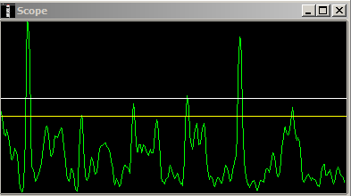
Looking at the FLDIGI signal scope below you can see the difference on noise level. Note that these were captured at different times so they represent different morse letters.  Figure 3 is without matched filter and figure 4 has matched filter enabled.  Reduction of noise is clearly visible.

Figure 3. Without Matched Filter

Figure 4. With Matched Filter

To enable testing Matched Filter I modified the FLDIGI Modems / CW / General configuration screen.  I added a checkbox and a "Matched Filter length" slider  that represents buffer length in 10ms units.  So  "227" in figure 5 below represents 2.27 second input buffer for the matched filter. The results improve the longer the buffer is set  but this also causes longer latency between the received audio and decoded characters appearing on the screen.  At 18 WPM morse speed  1...2 second delay seemed like a reasonable compromise. I set the range between  100ms and 3 seconds in the user interface. For longer messages such as bulletins even longer buffer could be applicable.

I am also using "Use Farnsworth timing" tick box to enable/disable SOM detection feature (I was lazy and did not want to create another tick box user interface). This enables to test SOM feature in real time and see if it makes any difference.

Figure 5.  Modified FLDIGI configuration screen

4) CONCLUSIONS

I implemented two new experimental features to FLDIGI software package, namely  Matched Filter  and Self Organizing Maps decoding.  My objective was to improve FLDIGI morse code detection and decoding capabilities.

Based on above testing  it seems that both detection and decoding capabilities improved  compared to baseline algorithms in FLDIGI.  However,  the testing above was done with artificially generated noisy morse signal, not with real life audio from noisy RF bands. I am planning to run more tests to verify how well these features work with real life cases.

These two experimental features could potentially be beneficial in the following areas: 

• Decoding morse signals with low signal-to-noise ratio such as in VHF / UHF / 50 Mhz bands  - combined with PSK reporter type functionality we could get automatic alerts on band openings,  such as Es or tropo, from FLDIGI 
• Monitoring weak CW beacons   
• Working with QRP stations 
• Perhaps even  working EME  QSOs  with smaller antennas

The software is alpha quality and not ready for broader distribution. Since I have only limited amount of time available I would like to collaborate with other hams who could help me to improve this software and hopefully make it ready for mainline FLDIGI distribution in future.

If you are able to compile FLDIGI from source tar files on Linux  and you don't need any support to resolve problems I can send the tar file via email.

5) ACKNOWLEGEMENT

I would like to express my gratitude to David H Freese, W1HKJ for making FLDIGI available as open source software.  This great software package is not only very useful piece of ham radio software but also a fantastic treasure trove of digital signal processing gems. 

I would also like to thank  Rob Frohne, KL7NA for making matched filter and many other algorithms publicly available for his students and providing great insights over multiple emails we have exchanged. 
 

73  de Mauri,  AG1LE